拷贝是Python学习过程中很容易被忽略,但是在项目开发过程中起着重要作用的一个概念。
有很多开发者由于忽视这一点,甚至导致项目中出现很严重的BUG。
我之前就因为这样的一个小问题,一不小心掉坑里了。反复定位才发现竟然是由这个容易被忽视的问题引起的….
在这篇文章中,我们将看看如何在Python中深度和浅度拷贝对象,深入探讨Python 如何处理对象引用和内存中的对象。
浅拷贝
当我们在 Python 中使用赋值语句 (=) 来创建复合对象的副本时,例如,列表或类实例或基本上任何包含其他对象的对象,Python 并没有克隆对象本身。
相反,它只是将引用绑定到目标对象上。
想象一下,我们有一个列表,里面有以下元素。
original_list =[[1,2,3], [4,5,6], ["X", "Y", "Z"]]如果我们尝试使用如下的赋值语句来复制我们的原始列表。
shallow_copy_list = original_list
print(shallow_copy_list)
它可能看起来像我们克隆了我们的对象,或许很多同学会认为生成了两个对象,
[[1,2,3], [4,5,6], ['X', 'Y', 'Z']]但是,我们真的有两个对象吗?
不,并没有。我们有两个引用变量,指向内存中的同一个对象。通过打印这两个对象在内存中的ID,可以很容易地验证这一点。
id(original_list) # 4517445712
id(shallow_copy_list) # 4517445712
一个更具体的证明可以通过尝试改变 “两个列表”中的一个值来观察–而实际上,我们改变的是同一个列表,两个指针指向内存中的同一个对象。
让我们来改变original_list所指向的对象的最后一个元素。
# Last element of last element
original_list[-1][-1] = "ZZZ"
print(original_list)
输出结果是:
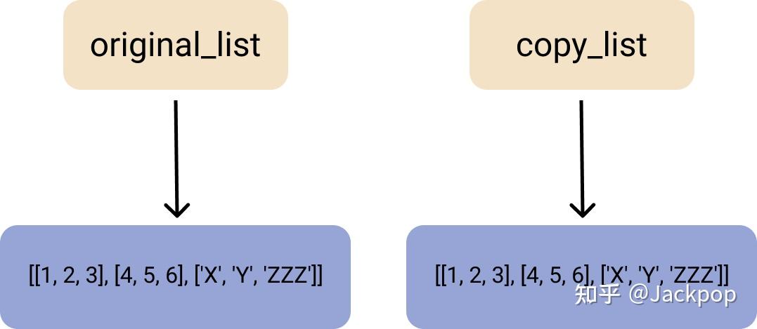
[[1, 2, 3], [4, 5, 6], ['X', 'Y', 'ZZZ']]两个引用变量都指向同一个对象,打印shallow_copy_list将返回相同的结果。
print(shallow_copy_list) # [[1, 2, 3], [4, 5, 6], ['X', 'Y', 'ZZZ']]浅层复制是指复制一个对象的引用并将其存储在一个新的变量中的过程。original_list和shallow_copy_list只是指向内存(RAM)中相同地址的引用,这些引用存储了[[1, 2, 3], [4, 5, 6], ['X', 'Y', 'ZZZ']的值。
我们在复制过程中,并没有生成一个新的对象,试想一下,如果不理解这一点,很多同学会误认为它生成了一个完全独立的新对象,殊不知,在对这个新变量shallow_copy_list进行操作时,原来的变量original_list也会跟随改变。
除了赋值语句之外,还可以通过Python标准库的拷贝模块实现浅拷贝
要使用拷贝模块,我们必须首先导入它。
import copy
second_shallow_copy_list = copy.copy(original_list)
把它们都打印出来,看看它们是否引用了相同的值。
print(original_list)
print(second_shallow_copy_list)
不出所料,确实如此,
[[1, 2, 3], [4, 5, 6], ['X', 'Y', 'ZZZ']]
[[1, 2, 3], [4, 5, 6], ['X', 'Y', 'ZZZ']]
通常,你想复制一个复合对象,例如在一个方法的开始,然后修改克隆的对象,但保持原始对象的原样,以便以后再使用它。
为了达到这个目的,我们需要对该对象进行深度复制。现在让我们来学习一下什么是深度拷贝以及如何深度拷贝一个复合对象。
深拷贝
深度复制一个对象意味着真正地将该对象和它的值克隆到内存中的一个新的副本(实例)中,并具有这些相同的值。
通过深度拷贝,我们实际上可以创建一个独立于原始数据的新对象,但包含相同的值,而不是为相同的值创建新的引用。
在一个典型的深度拷贝过程中,首先,一个新的对象引用被创建,然后所有的子对象被递归地加入到父对象中。
这样一来,与浅层拷贝不同,对原始对象的任何修改都不会反映在拷贝对象中(反之亦然)。
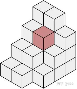
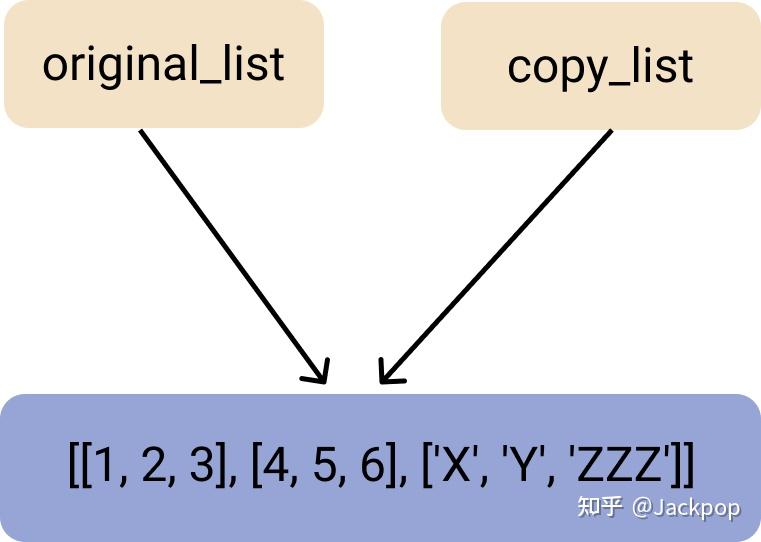
下面是一个典型的深度拷贝的简单图示。
要在 Python 中深度拷贝一个对象,我们使用 copy 模块的 deepcopy()方法。
让我们导入 copy 模块并创建一个列表的深度拷贝。
import copy

original_list = [[1,2,3], [4,5,6], ["X", "Y", "Z"]]
deepcopy_list = copy.deepcopy(original_list)
现在让我们打印我们的列表,以确保输出是相同的,以及他们的ID是唯一的。
print(id(original_list), original_list)
print(id(deepcopy_list), deepcopy_list)
输出结果证实,我们已经为自己创建了一个真正的副本。
4517599280, [[1, 2, 3], [4, 5, 6], ['X', 'Y', 'Z']]
4517599424, [[1, 2, 3], [4, 5, 6], ['X', 'Y', 'Z']]
现在让我们试着修改我们的原始列表,把最后一个列表的最后一个元素改为 “O”,然后打印出来看看结果。
original_list[-1][-1] = "O"
print(original_list)
我们得到了预期的结果。
[[1, 2, 3], [4, 5, 6], ['X', 'Y', 'O']]现在,如果我们继续前进并尝试打印我们的副本列表,之前的修改并没有影响新的变量。
print(deepcopy_list) # [[1, 2, 3], [4, 5, 6], ['X', 'Y', 'Z']]记住,copy()和deepcopy()方法适用于其他复合对象。这意味着,你也可以用它们来创建类实例的副本。