YOLO系列(四):yolov3

yolov3属于一阶段、anchor-based 目标检测

FPN :

原来多数的object detection算法都是只采用顶层特征做预测,但我们知道低层的特征语义信息比较少,但是目标位置准确;高层的特征语义信息比较丰富,但是目标位置比较粗略。另外虽然也有些算法采用多尺度特征融合的方式,但是一般是采用融合后的特征做预测,而本文不一样的地方在于预测是在不同特征层独立进行的。

FPN(Feature Pyramid Network)算法可以同时利用低层特征高分辨率和高层特征的高语义信息,通过融合这些不同层的特征达到很好的预测效果。此外,和其他的特征融合方式不同的是本文中的预测是在每个融合后的特征层上单独进行的。(对不同特征层单独预测)

网络结构解析:

  1. Yolov3中,只有卷积层,通过调节卷积步长控制输出特征图的尺寸。所以对于输入图片尺寸没有特别限制。流程图中,输入图片以256*256作为样例。
  2. Yolov3借鉴了金字塔特征图思想,小尺寸特征图用于检测大尺寸物体,而大尺寸特征图检测小尺寸物体。特征图的输出维度为 [公式] , [公式] 为输出特征图格点数,一共3个Anchor框,每个框有4维预测框数值 [公式] ,1维预测框置信度,80维物体类别数。所以第一层特征图的输出维度为 [公式] 。
  3. Yolov3总共输出3个特征图,第一个特征图下采样32倍,第二个特征图下采样16倍,第三个下采样8倍。输入图像经过Darknet-53(无全连接层),再经过Yoloblock生成的特征图被当作两用,第一用为经过3*3卷积层、1*1卷积之后生成特征图一,第二用为经过1*1卷积层加上采样层,与Darnet-53网络的中间层输出结果进行拼接,产生特征图二。同样的循环之后产生特征图三。
  4. concat操作与加和操作的区别:加和操作来源于ResNet思想,将输入的特征图,与输出特征图对应维度进行相加,即 [公式] ;而concat操作源于DenseNet网络的设计思路,将特征图按照通道维度直接进行拼接,例如8*8*16的特征图与8*8*16的特征图拼接后生成8*8*32的特征图。
  5. 上采样层(upsample):作用是将小尺寸特征图通过插值等方法,生成大尺寸图像。例如使用最近邻插值算法,将8*8的图像变换为16*16。上采样层不改变特征图的通道数。

Yolo的整个网络,吸取了Resnet、Densenet、FPN的精髓,可以说是融合了目标检测当前业界最有效的全部技巧。

YOLOv3网络结构示意图(VOC数据集)
YOLOv3所用的Darknet-53模型

YOLO系列(三):yolov2

yolov2属于一阶段、anchor-based 目标检测

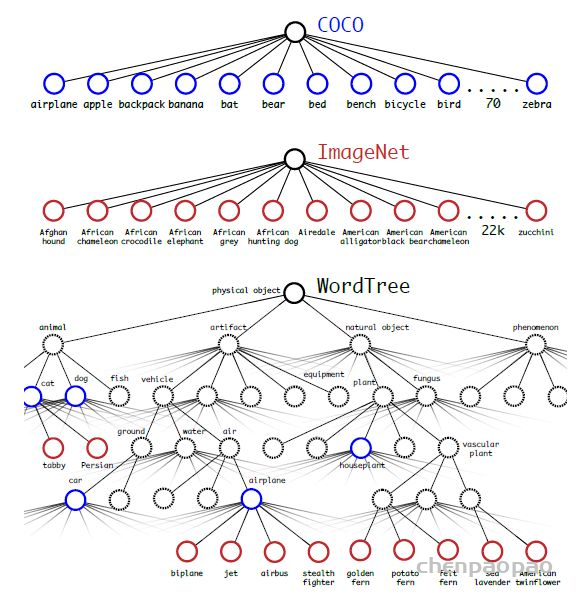
YOLOv2的论文全名为YOLO9000: Better, Faster, Stronger,它斩获了CVPR 2017 Best Paper Honorable Mention。在这篇文章中,作者首先在YOLOv1的基础上提出了改进的YOLOv2,然后提出了一种检测与分类联合训练方法,使用这种联合训练方法在COCO检测数据集和ImageNet分类数据集上训练出了YOLO9000模型,其可以检测超过9000多类物体。所以,这篇文章其实包含两个模型:YOLOv2和YOLO9000,不过后者是在前者基础上提出的,两者模型主体结构是一致的。YOLOv2相比YOLOv1做了很多方面的改进,这也使得YOLOv2的mAP有显着的提升,并且YOLOv2的速度依然很快,保持着自己作为one-stage方法的优势.

Yolov2和Yolo9000算法内核相同,区别是训练方式不同:Yolov2用coco数据集训练后,可以识别80个种类。而Yolo9000可以使用coco数据集 + ImageNet数据集联合训练,可以识别9000多个种类。

YOLOv2的改进策略

YOLOv1虽然检测速度很快,但是在检测精度上却不如R-CNN系检测方法,YOLOv1在物体定位方面(localization)不够准确,并且召回率(recall)较低。YOLOv2共提出了几种改进策略来提升YOLO模型的定位准确度和召回率,从而提高mAP,YOLOv2在改进中遵循一个原则:保持检测速度,这也是YOLO模型的一大优势。YOLOv2的改进策略如图2所示,可以看出,大部分的改进方法都可以比较显着提升模型的mAP。

Batch Normalization

Batch Normalization可以提升模型收敛速度,而且可以起到一定正则化效果,降低模型的过拟合。在YOLOv2中,每个卷积层后面都添加了Batch Normalization层,并且不再使用droput。使用Batch Normalization后,YOLOv2的mAP提升了2.4%。

High Resolution Classifier:

目前大部分的检测模型都会在先在ImageNet分类数据集上预训练模型的主体部分(CNN特征提取器),由于历史原因,ImageNet分类模型基本采用大小为 224*224的图片作为输入,分辨率相对较低,不利于检测模型。所以YOLOv1在采用 224*224 分类模型预训练后,将分辨率增加至 448*448,并使用这个高分辨率在检测数据集上finetune。但是直接切换分辨率,检测模型可能难以快速适应高分辨率。所以YOLOv2增加了在ImageNet数据集上使用448*448输入来finetune分类网络这一中间过程(10 epochs),这可以使得模型在检测数据集上finetune之前已经适用高分辨率输入。使用高分辨率分类器后,YOLOv2的mAP提升了约4%。

Convolutional With Anchor Boxes:在YOLOv1中,输入图片最终被划分为7*7网格,每个单元格预测2个边界框。YOLOv1最后采用的是全连接层直接对边界框进行预测,其中边界框的宽与高是相对整张图片大小的,而由于各个图片中存在不同尺度和长宽比(scales and ratios)的物体,YOLOv1在训练过程中学习适应不同物体的形状是比较困难的,这也导致YOLOv1在精确定位方面表现较差。YOLOv2借鉴了Faster R-CNN中RPN网络的先验框(anchor boxes,prior boxes,SSD也采用了先验框)策略。RPN对CNN特征提取器得到的特征图(feature map)进行卷积来预测每个位置的边界框以及置信度(是否含有物体),并且各个位置设置不同尺度和比例的先验框,所以RPN预测的是边界框相对于先验框的offsets值(其实是transform值,详细见Faster R_CNN论文),采用先验框使得模型更容易学习。所以YOLOv2移除了YOLOv1中的全连接层而采用了卷积和anchor boxes来预测边界框。为了使检测所用的特征图分辨率更高,移除其中的一个pool层。在检测模型中,YOLOv2不是采用448*448图片作为输入,而是采用416*416大小。因为YOLOv2模型下采样的总步长为32,对于 416*416 大小的图片,最终得到的特征图大小为 13*13,维度是奇数,这样特征图恰好只有一个中心位置。对于一些大物体,它们中心点往往落入图片中心位置,此时使用特征图的一个中心点去预测这些物体的边界框相对容易些。所以在YOLOv2设计中要保证最终的特征图有奇数个位置。对于YOLOv1,每个cell都预测2个boxes,每个boxes包含5个值: (x,y,w,h,c),前4个值是边界框位置与大小,最后一个值是置信度(confidence scores,包含两部分:含有物体的概率以及预测框与ground truth的IOU)。但是每个cell只预测一套分类概率值(class predictions,其实是置信度下的条件概率值),供2个boxes共享。YOLOv2使用了anchor boxes之后,每个位置的各个anchor box都单独预测一套分类概率值,这和SSD比较类似(但SSD没有预测置信度,而是把background作为一个类别来处理)。使用anchor boxes之后,YOLOv2的mAP有稍微下降(这里下降的原因,我猜想是YOLOv2虽然使用了anchor boxes,但是依然采用YOLOv1的训练方法YOLOv1只能预测98个边界框( 7*7*2 ),而YOLOv2使用anchor boxes之后可以预测上千个边界框(13*13*num_anchors)。所以使用anchor boxes之后,YOLOv2的召回率大大提升,由原来的81%升至88%。

Dimension Clusters

在Faster R-CNN和SSD中,先验框的维度(长和宽)都是手动设定的,带有一定的主观性。如果选取的先验框维度比较合适,那么模型更容易学习,从而做出更好的预测。因此,YOLOv2采用k-means聚类方法对训练集中的边界框做了聚类分析。因为设置先验框的主要目的是为了使得预测框与ground truth的IOU更好,所以聚类分析时选用box与聚类中心box之间的IOU值作为距离指标:

$$
d(\text { box }, \text { centroid })=1-I O U(\text { box }, \text { centroid })
$$

下图为在VOC和COCO数据集上的聚类分析结果,随着聚类中心数目的增加,平均IOU值(各个边界框与聚类中心的IOU的平均值)是增加的,但是综合考虑模型复杂度和召回率,作者最终选取5个聚类中心作为先验框,其相对于图片的大小如右边图所示。对于两个数据集,5个先验框的width和height如下所示(来源:YOLO源码的cfg文件):

COCO: (0.57273, 0.677385), (1.87446, 2.06253), (3.33843, 5.47434), (7.88282, 3.52778), (9.77052, 9.16828)
VOC: (1.3221, 1.73145), (3.19275, 4.00944), (5.05587, 8.09892), (9.47112, 4.84053), (11.2364, 10.0071)

但是这里先验框的大小具体指什么作者并没有说明,但肯定不是像素点,从代码实现上看,应该是相对于预测的特征图大小( [公式] )。对比两个数据集,也可以看到COCO数据集上的物体相对小点。这个策略作者并没有单独做实验,但是作者对比了采用聚类分析得到的先验框与手动设置的先验框在平均IOU上的差异,发现前者的平均IOU值更高,因此模型更容易训练学习。

图3:数据集VOC和COCO上的边界框聚类分析结果

New Network: Darknet-19

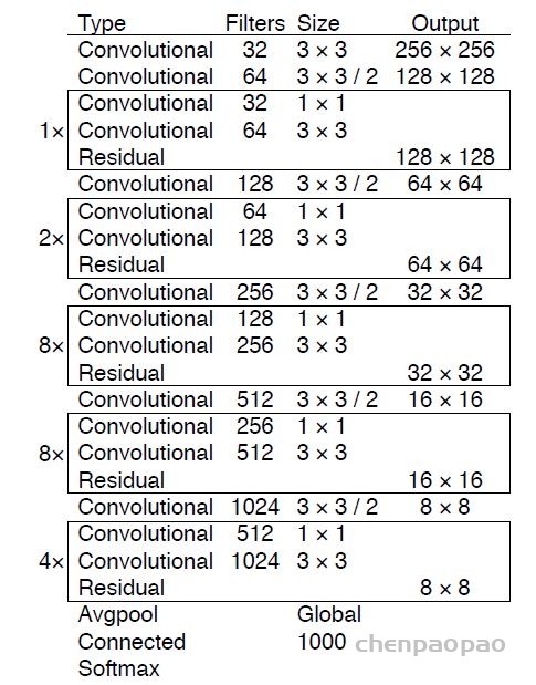
YOLOv2采用了一个新的基础模型(特征提取器),称为Darknet-19,包括19个卷积层和5个maxpooling层,如图4所示。Darknet-19与VGG16模型设计原则是一致的,主要采用3*3卷积,采用2*2的maxpooling层之后,特征图维度降低2倍,而同时将特征图的channles增加两倍。与NIN(Network in Network)类似,Darknet-19最终采用global avgpooling做预测,并且在3*3卷积之间使用1*1卷积来压缩特征图channles以降低模型计算量和参数。Darknet-19每个卷积层后面同样使用了batch norm层以加快收敛速度,降低模型过拟合。在ImageNet分类数据集上,Darknet-19的top-1准确度为72.9%,top-5准确度为91.2%,但是模型参数相对小一些。使用Darknet-19之后,YOLOv2的mAP值没有显着提升,但是计算量却可以减少约33%。

Direct location prediction

沿用YOLOv1的方法,就是预测边界框中心点相对于对应cell左上角位置的相对偏移值,为了将边界框中心点约束在当前cell中,使用sigmoid函数处理偏移值,这样预测的偏移值在(0,1)范围内(每个cell的尺度看做1)。

Fine-Grained Features 更精细的特征图

YOLOv2的输入图片大小为 416*416 ,经过5次maxpooling之后得到 13*13 大小的特征图,并以此特征图采用卷积做预测。13*13大小的特征图对检测大物体是足够了,但是对于小物体还需要更精细的特征图(Fine-Grained Features)。因此SSD使用了多尺度的特征图来分别检测不同大小的物体,前面更精细的特征图可以用来预测小物体。YOLOv2提出了一种passthrough层来利用更精细的特征图。YOLOv2所利用的Fine-Grained Features是26*26大小的特征图(最后一个maxpooling层的输入),对于Darknet-19模型来说就是大小为 26*26*512 的特征图。passthrough层与ResNet网络的shortcut类似,以前面更高分辨率的特征图为输入,然后将其连接到后面的低分辨率特征图上。前面的特征图维度是后面的特征图的2倍,passthrough层抽取前面层的每个 2*2的局部区域,然后将其转化为channel维度,对于 [ 26*26*512 ] 的特征图,经passthrough层处理之后就变成了 [13*13*2048] 的新特征图(特征图大小降低4倍,而channles增加4倍,下图为一个实例),这样就可以与后面的 [13*13*1024] 特征图连接在一起形成 13*13*3072大小的特征图,然后在此特征图基础上卷积做预测。在YOLO的C源码中,passthrough层称为reorg layer。在TensorFlow中,可以使用tf.extract_image_patches或者tf.space_to_depth来实现passthrough层

passthrough层实例

Multi-Scale Training

采用Multi-Scale Training策略,YOLOv2可以适应不同大小的图片,并且预测出很好的结果。在测试时,YOLOv2可以采用不同大小的图片作为输入,在VOC 2007数据集上的效果如下图所示。可以看到采用较小分辨率时,YOLOv2的mAP值略低,但是速度更快,而采用高分辨输入时,mAP值更高,但是速度略有下降,对于 544*544,mAP高达78.6%。注意,这只是测试时输入图片大小不同,而实际上用的是同一个模型(采用Multi-Scale Training训练)

YOLO9000

YOLO9000是在YOLOv2的基础上提出的一种可以检测超过9000个类别的模型,其主要贡献点在于提出了一种分类和检测的联合训练策略。众多周知,检测数据集的标注要比分类数据集打标签繁琐的多,所以ImageNet分类数据集比VOC等检测数据集高出几个数量级。在YOLO中,边界框的预测其实并不依赖于物体的标签,所以YOLO可以实现在分类和检测数据集上的联合训练。对于检测数据集,可以用来学习预测物体的边界框、置信度以及为物体分类,而对于分类数据集可以仅用来学习分类,但是其可以大大扩充模型所能检测的物体种类。

作者选择在COCO和ImageNet数据集上进行联合训练,但是遇到的第一问题是两者的类别并不是完全互斥的,比如”Norfolk terrier”明显属于”dog”,所以作者提出了一种层级分类方法(Hierarchical classification),主要思路是根据各个类别之间的从属关系(根据WordNet)建立一种树结构WordTree

WordTree中的根节点为”physical object”,每个节点的子节点都属于同一子类,可以对它们进行softmax处理。在给出某个类别的预测概率时,需要找到其所在的位置,遍历这个path,然后计算path上各个节点的概率之积。

在训练时,如果是检测样本,按照YOLOv2的loss计算误差,而对于分类样本,只计算分类误差。在预测时,YOLOv2给出的置信度就是 [公式] ,同时会给出边界框位置以及一个树状概率图。在这个概率图中找到概率最高的路径,当达到某一个阈值时停止,就用当前节点表示预测的类别。

通过联合训练策略,YOLO9000可以快速检测出超过9000个类别的物体,总体mAP值为19,7%。我觉得这是作者在这篇论文作出的最大的贡献,因为YOLOv2的改进策略亮点并不是很突出,但是YOLO9000算是开创之举。

reference:

https://zhuanlan.zhihu.com/p/35325884

SSD原理与实现

SSD属于一阶段、anchor-based 目标检测

基于anchor-based的技术包括一个阶段和两个阶段的检测。其中一阶段的检测技术包括SSD,DSSD,RetinaNet,RefineDet,YOLOV3等,二阶段技术包括Faster-RCNN,R-FCN,FPN,Cascade R-CNN,SNIP等。一般的,两个阶段的目标检测会比一个阶段的精度要高,但一个阶段的算法速度会更快。

 anchor-based类算法代表是fasterRCNN、SSD、YoloV2/V3等

目标检测近年来已经取得了很重要的进展,主流的算法主要分为两个类型(参考RefineDet):(1)two-stage方法,如R-CNN系算法,其主要思路是先通过启发式方法(selective search)或者CNN网络(RPN)产生一系列稀疏的候选框,然后对这些候选框进行分类与回归,two-stage方法的优势是准确度高;(2)one-stage方法,如Yolo和SSD,其主要思路是均匀地在图片的不同位置进行密集抽样,抽样时可以采用不同尺度和长宽比,然后利用CNN提取特征后直接进行分类与回归,整个过程只需要一步,所以其优势是速度快,但是均匀的密集采样的一个重要缺点是训练比较困难,这主要是因为正样本与负样本(背景)极其不均衡(参见Focal Loss),导致模型准确度稍低。

需要掌握的知识:

1、边界框

在⽬标检测中,我们通常使⽤边界框(bounding box)来描述对象的空间位置。边界框是矩形的,由矩形左上⻆的 x 和 y 坐标以及右下⻆的坐标决定。另⼀种常⽤的边界框表⽰⽅法是边界框中⼼的 (x, y) 轴坐标以及框的宽度和⾼度

2、锚框

⽬标检测算法通常会在输⼊图像中采样⼤量的区域,然后判断这些区域中是否包含我们感兴趣的⽬标,并调整区域边缘从而更准确地预测⽬标的真实边界框(ground-truth bounding box)。不同的模型使⽤的区域采样⽅法可能不同。这⾥我们介绍其中的⼀种⽅法:它以每个像素为中⼼⽣成多个⼤小和宽⾼⽐(aspect ratio)不同的边界框。这些边界框被称为锚框(anchor box)

3、交并⽐(IoU)

直观地说,我们可以衡量锚框和真实边界框之间的相似性。我们知道 Jaccard 系数可以衡量
两组之间的相似性。给定集合 A 和 B,他们的 Jaccard 系数是他们交集的⼤小除以他们并集的⼤小:$$J\left( A,B\right) =\dfrac{\left| A\cap B\right| }{\left| A\right| U\left| B\right| }$$ 事实上,我们可以将任何边界框的像素区域视为⼀组像素。通过这种⽅式,我们可以通过其像素集的 Jaccard索引来测量两个边界框的相似性。对于两个边界框,我们通常将他们的 Jaccard 指数称为 交并⽐ (intersectionover union,IoU),即两个边界框相交⾯积与相并⾯积之⽐

4、标注训练数据的锚框

在训练集中,我们将每个锚框视为⼀个训练样本。为了训练⽬标检测模型,我们需要每个锚框的类别(class)和偏移量(offset)标签,其中前者是与锚框相关的对象的类别,后者是真实边界框相对于锚框的偏移量。在预测期间,我们为每个图像⽣成多个锚框,预测所有锚框的类和偏移量,根据预测的偏移量调整它们的位置以获得预测的边界框,最后只输出符合特定条件的预测边界框。

5、将真实边界框分配给锚框

给定图像, 假设锚框是 \(A_{1}, A_{2}, \ldots, A_{n_{a}}\) , 真实边界框是 \(B_{1}, B_{2}, \ldots, B_{n_{b}}\) , 其中 \( n_{a} \geq n_{b}\) 。让我们定义一个矩 阵 \(\mathbf{X} \in \mathbb{R}^{n_{a} \times n_{b}}\), 其中 \(i^{\text {th }}\) 行和 \(j^{\text {th }}\) 列中的元素 \(x_{i j}\)是针框 \(A_{i}\) 和真实边界框 \(B_{j}\) 的 \(\mathrm{IoU}\) 。该算法包含以下步骤:

  1. 在矩阵 \(\mathbf{X}\) 中找到最大的元素, 并将它的行索引和列索引分别表示为 \(i_{1}\) 和 \(j_{1}\) 。然后将真实边界框 \(B_{j_{1}}\) 分 配给针框 \(A_{i_{1}}\) 。这很直观,因为 \(A_{i_{1}}\) 和 \(B_{j_{1}}\) 是所有针框和真实边界框配对中最相近的。在第一个分配完 成后,丢弃矩阵中 \(i_{1}{ }^{\text {th }}\) 行和 \(j_{1}{ }^{\text {th }}\) 列中的所有元素。
  2. 在矩阵 \(\mathbf{X}\) 中找到剩余元素中最大的元素, 并将它的行索引和列索引分别表示为 \(i_{2}\) 和 \(j_{2}\) 。我们将真实边 界框 \(B_{j_{2}}\) 分配给针框 \(A_{i_{2}}\), 并丢弃矩阵中 \(i_{2}{ }^{\text {th }}\) 行和 \(j_{2}{ }^{\text {th }}\) 列中的所有元素。
  3. 此时,矩阵 \(\mathbf{X}\) 中两行和两列中的元素已被丢弃。我们继续, 直到丢弃掉矩阵 \(\mathbf{X}\) 中 \(n_{b}\) 列中的所有元素。 此时,我们已经为这 \(n_{b}\) 个针框各自分配了一个真实边界框。
  4. 只遍历剩下的 \(n_{a}-n_{b}\) 个针框。例如,给定任何针框 \(A_{i}\), 在矩阵 \(\mathbf{X}\)的第 \(i^{\text {th }}\) 行中找到与 \(A_{i}\) 的IoU最大的 真实边界框 \(B_{j}\), 只有当此 IoU 大于预定义的阈值时, 才将 \(B_{j}\) 分配给 \(A_{i \circ}\)

6、标记类和偏移

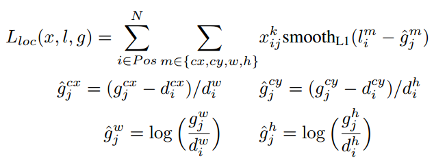
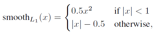
现在我们可以为每个锚框标记分类和偏移量了。假设⼀个锚框 A 被分配了⼀个真实边界框 B。⼀⽅⾯,锚框A 的类将被标记为与 B 相同。另⼀⽅⾯,锚框 A 的偏移量将根据 B 和 A 中⼼坐标的相对位置、以及这两个框的相对⼤小进⾏标记。鉴于数据集内不同的框的位置和⼤小不同,我们可以对那些相对位置和⼤小应⽤变换,使其获得更均匀分布、易于适应的偏移量。在这⾥,我们介绍⼀种常⻅的变换。给定框 A 和 B,中⼼坐标分别为 (xa, ya) 和 (xb, yb),宽度分别为 wa 和 wb,⾼度分别为 ha 和 hb。我们可以将 A 的偏移量标记为

$$
\left(\frac{\frac{x_{b}-x_{a}}{w_{a}}-\mu_{x}}{\sigma_{x}}, \frac{\frac{y_{b}-y_{a}}{h_{a}}-\mu_{y}}{\sigma_{y}}, \frac{\log \frac{w_{b}}{w_{a}}-\mu_{w}}{\sigma_{w}}, \frac{\log \frac{h_{b}}{h_{a}}-\mu_{h}}{\sigma_{h}}\right)
$$

$$
\text { 其中常量的默认值是 } \mu_{x}=\mu_{y}=\mu_{w}=\mu_{h}=0, \sigma_{x}=\sigma_{y}=0.1 \text { 和 } \sigma_{w}=\sigma_{h}=0.2 \text { 。 }
$$

7、⽤⾮极⼤值抑制预测边界框

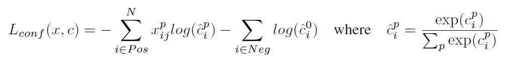
在预测期间,我们先为图像⽣成多个锚框,再为这些锚框⼀⼀预测类别和偏移量。⼀个“预测好的边界框”则根据其中某个带有预测偏移量的锚框而⽣成。当有许多锚框时,可能会输出许多相似的具有明显重叠的预测边界框,都围绕着同⼀⽬标。为了简化输出,我们可以使⽤ ⾮极⼤值抑制 (non-maximum suppression,NMS)合并属于同⼀⽬标的类似的预测边界框。以下是⾮极⼤值抑制的⼯作原理。对于⼀个预测边界框 B,⽬标检测模型会计算每个类的预测概率。假设最⼤的预测概率为 p ,则该概率所对应的类别 B 即为预测的类别。具体来说,我们将 p 称为预测边界框 B 的置信度。在同⼀张图像中,所有预测的⾮背景边界框都按置信度降序排序,以⽣成列表 L。然后我们通过以下步骤操作排序列表 L:

  1. 从 L 中选取置信度最高的预测边界框 \(B_{1}\) 作为基准,然后将所有与 \(B_{1}\) 的IoU 超过预定阈值\(\epsilon\) 的非基准 预测边界框从 L 中移除。这时, L 保留了置信度最高的预测边界框,去除了与其太过相似的其他预测 边界框。简而言之,那些具有 非极大值置信度的边界框被 抑制了。
  2. 从 L 中选取置信度第二高的预测边界框 \(B_{2}\) 作为又一个基准,然后将所有与 \(B_{2}\)的IoU大于 \(\epsilon\)的非基准 预测边界框从 L 中移除。
  3. 重复上述过程,直到 L 中的所有预测边界框都曾被用作基准。此时, L中任意一对预测边界框的IoU都 小于阈值 \(\epsilon\); 因此,没有一对边界框过于相似。
  4. 输出列表 L中的所有预测边界框。

SSD原理:

在了解上述概念后,开始实现SSD(Single Shot MultiBox Detector)

SSD和Yolo一样都是采用一个CNN网络来进行检测,但是却采用了多尺度的特征图,其基本架构如图3所示。下面将SSD核心设计理念总结为以下三点:

(1)采用多尺度特征图用于检测

所谓多尺度采用大小不同的特征图,CNN网络一般前面的特征图比较大,后面会逐渐采用stride=2的卷积或者pool来降低特征图大小,这正如图3所示,一个比较大的特征图和一个比较小的特征图,它们都用来做检测。这样做的好处是比较大的特征图来用来检测相对较小的目标,而小的特征图负责检测大目标。

(2)采用卷积进行检测

与Yolo最后采用全连接层不同,SSD直接采用卷积对不同的特征图来进行提取检测结果。对于形状为 [公式] 的特征图,只需要采用 [公式] 这样比较小的卷积核得到检测值。

(3)设置先验框

在Yolo中,每个单元预测多个边界框,但是其都是相对这个单元本身(正方块),但是真实目标的形状是多变的,Yolo需要在训练过程中自适应目标的形状。而SSD借鉴了Faster R-CNN中anchor的理念,每个单元设置尺度或者长宽比不同的先验框预测的边界框(bounding boxes)是以这些先验框为基准的,在一定程度上减少训练难度。一般情况下,每个单元会设置多个先验框,其尺度和长宽比存在差异,如图5所示,可以看到每个单元使用了4个不同的先验框,图片中猫和狗分别采用最适合它们形状的先验框来进行训练,后面会详细讲解训练过程中的先验框匹配原则

也就是说,在上面4中所说的 “标注训练数据的锚框” ,这里的 框在SSD中就是先验框。

网络结构

SSD采用VGG16作为基础模型,然后在VGG16的基础上新增了卷积层来获得更多的特征图以用于检测。SSD的网络结构如图5所示。上面是SSD模型,下面是Yolo模型,可以明显看到SSD利用了多尺度的特征图做检测。

得到了特征图之后,需要对特征图进行卷积得到检测结果

下图给出了一个 5*5大小的特征图的检测过程。其中Priorbox是得到先验框,前面已经介绍了生成规则。检测值包含两个部分:类别置信度和边界框位置,各采用一次3*3 卷积来进行完成。

训练过程

(1)先验框匹配
在训练过程中,首先要确定训练图片中的ground truth(真实目标)与哪个先验框来进行匹配,与之匹配的先验框所对应的边界框将负责预测它。在Yolo中,ground truth的中心落在哪个单元格,该单元格中与其IOU最大的边界框负责预测它。但是在SSD中却完全不一样,SSD的先验框与ground truth的匹配原则主要有两点。首先,对于图片中每个ground truth,找到与其IOU最大的先验框,该先验框与其匹配,这样,可以保证每个ground truth一定与某个先验框匹配。通常称与ground truth匹配的先验框为正样本(其实应该是先验框对应的预测box,不过由于是一一对应的就这样称呼了),反之,若一个先验框没有与任何ground truth进行匹配,那么该先验框只能与背景匹配,就是负样本。一个图片中ground truth是非常少的, 而先验框却很多,如果仅按第一个原则匹配,很多先验框会是负样本,正负样本极其不平衡,所以需要第二个原则。第二个原则是:对于剩余的未匹配先验框,若某个ground truth的 IOU大于某个阈值(一般是0.5),那么该先验框也与这个ground truth进行匹配。这意味着某个ground truth可能与多个先验框匹配,这是可以的。但是反过来却不可以,因为一个先验框只能匹配一个ground truth,如果多个ground truth与某个先验框 IOU大于阈值,那么先验框只与IOU最大的那个ground truth进行匹配。第二个原则一定在第一个原则之后进行,仔细考虑一下这种情况,如果某个ground truth所对应最大 IOU小于阈值,并且所匹配的先验框却与另外一个ground truth的IOU大于阈值,那么该先验框应该匹配谁,答案应该是前者,首先要确保某个ground truth一定有一个先验框与之匹配。但是,这种情况我觉得基本上是不存在的。由于先验框很多,某个ground truth的最大 IOU肯定大于阈值,所以可能只实施第二个原则既可以了,这里的TensorFlow版本就是只实施了第二个原则,但是这里的Pytorch两个原则都实施了

(2)损失函数
训练样本确定了,然后就是损失函数了。损失函数定义为位置误差(locatization loss, loc)与置信度误差(confidence loss, conf)的加权和:

$$
L(x, c, l, g)=\frac{1}{N}\left(L_{c o n f}(x, c)+\alpha L_{l o c}(x, l, g)\right)
$$
其中 N是先验框的正样本数量。这里\(x_{i j}^{p} \in{1,0}\) 为一个指示参数,当 \(x_{i j}^{p}=1\)时表示第 i 个先验框与第 j 个ground truth匹配,并且ground truth的类别为 p 。 c 为类别置信度预 测值。 l为先验框的所对应边界框的位置预测值,而 g 是ground truth的位置参数。对于位置误 差,其采用Smooth L1 loss,定义如下:

对于置信度误差,其采用softmax loss:

⽬标检测有两种类型的损失。第⼀种有关锚框类别的损失:我们可以简单地重⽤之前图像分类问题⾥⼀直使⽤的交叉熵损失函数来计算;第⼆种有关正类锚框偏移量的损失:预测偏移量是⼀个回归问题, 使⽤ L1 范数损失,即预测值和真实值之差的绝对值

3)数据扩增

采用数据扩增(Data Augmentation)可以提升SSD的性能,主要采用的技术有水平翻转(horizontal flip),随机裁剪加颜色扭曲(random crop & color distortion),随机采集块域(Randomly sample a patch)(获取小目标训练样本)

预测过程

预测过程比较简单,对于每个预测框,首先根据类别置信度确定其类别(置信度最大者)与置信度值,并过滤掉属于背景的预测框。然后根据置信度阈值(如0.5)过滤掉阈值较低的预测框。对于留下的预测框进行解码,根据先验框得到其真实的位置参数(解码后一般还需要做clip,防止预测框位置超出图片)。解码之后,一般需要根据置信度进行降序排列,然后仅保留top-k(如400)个预测框。最后就是进行NMS算法,过滤掉那些重叠度较大的预测框。最后剩余的预测框就是检测结果了。

性能评估

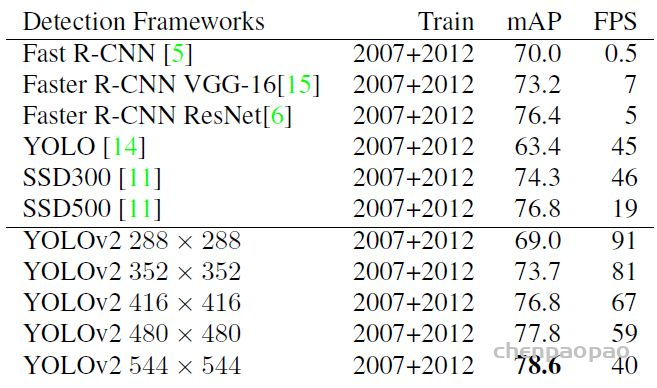
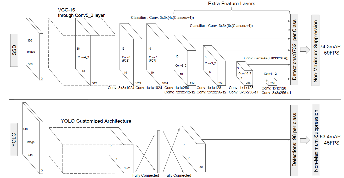
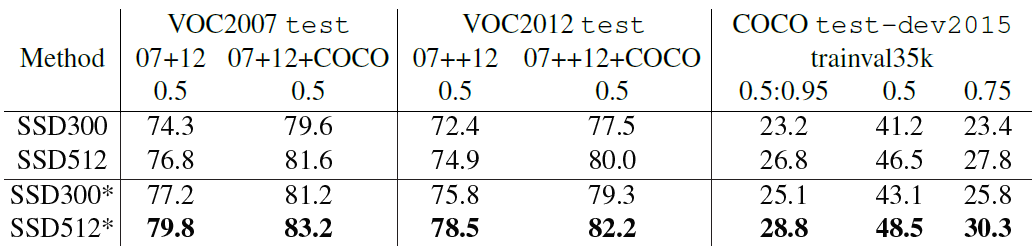
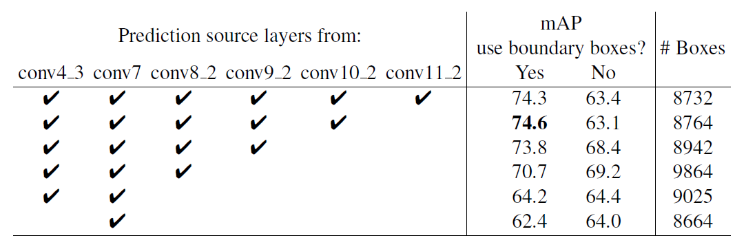
首先整体看一下SSD在VOC2007,VOC2012及COCO数据集上的性能,如表1所示。相比之下,SSD512的性能会更好一些。加*的表示使用了image expansion data augmentation(通过zoom out来创造小的训练样本)技巧来提升SSD在小目标上的检测效果,所以性能会有所提升。

表1 SSD在不同数据集上的性能

SSD与其它检测算法的对比结果(在VOC2007数据集)如表2所示,基本可以看到,SSD与Faster R-CNN有同样的准确度,并且与Yolo具有同样较快地检测速度。

表2 SSD与其它检测算法的对比结果(在VOC2007数据集)

文章还对SSD的各个trick做了更为细致的分析,表3为不同的trick组合对SSD的性能影响,从表中可以得出如下结论:

  • 数据扩增技术很重要,对于mAP的提升很大;
  • 使用不同长宽比的先验框可以得到更好的结果;
表3 不同的trick组合对SSD的性能影响

同样的,采用多尺度的特征图用于检测也是至关重要的,这可以从表4中看出:

表4 多尺度特征图对SSD的影响

参考: https://zhuanlan.zhihu.com/p/33544892

KL散度(相对熵)

定义:

若P和Q是定义在同一概率空间的两个概率测度,定义P和Q的相对熵为:

$$D\left( P\| Q\right) =\sum _{x}P\left( x\right) \log \dfrac{p\left( x\right) }{Q\left( x\right) }$$

性质:\( D\left( P\| Q\right) \) >=0

  在概率论或信息论中,KL散度( Kullback–Leibler divergence),又称相对熵(relative entropy),是描述两个概率分布P和Q差异的一种方法。它是非对称的,这意味着D(P||Q) ≠ D(Q||P)。特别的,在信息论中,D(P||Q)表示当用概率分布Q来拟合真实分布P时,产生的信息损耗,其中P表示真实分布,Q表示P的拟合分布。有人将KL散度称为KL距离,但事实上,KL散度并不满足距离的概念,应为:1)KL散度不是对称的;2)KL散度不满足三角不等式。

KL散度在信息论中有自己明确的物理意义,它是用来度量使用基于Q分布的编码来编码来自P分布的样本平均所需的额外的Bit个数。而其在机器学习领域的物理意义则是用来度量两个函数的相似程度或者相近程度.

基于P的编码去编码来自P的样本,其最优编码平均所需要的比特个数(即这个字符集的熵)为:

$$H\left( x\right) =\sum _{x}P\left( x\right) \log \left( \dfrac{1}{p\left( x\right) }\right)$$

用基于P的编码去编码来自Q的样本,则所需要的比特个数变为:

$$H’\left( x\right) =\sum _{x}P\left( x\right) \log \left( \dfrac{1}{Q\left( x\right) }\right)$$

于是,我们即可得出P与Q的KL散度:

$$D\left( P\| Q\right) = H\left( x\right) -H’\left( x\right)$$

图像金字塔pyrUp和pyrDown

函数作用:
图像金字塔中的向上和向下采样分别通过 pyrUp 和 pyrDown 实现。这里的向上向下采样,是针对图像的尺寸而言的(和金字塔的方向相反),向上就是图像尺寸加倍,向下就是图像尺寸减半。
对于 pyrUp,图像首先在每个维度上扩大为原来的两倍,新增的行和列(偶数行和列)以 0 填充。然后用指定的滤波器进行卷积(实际上是一个在每个维度上都扩大为原来两倍的过滤器)去估计”丢失“像素的近似值。
对于 pyrDown,先用高斯核对图像进行卷积,然后删除所有偶数行和偶数列,新的到的图像面积就会变成源图像的四分之一。
注意:pyrUp 和 pyrDown 不是互逆的。

通常,我们过去使用的是恒定大小的图像。但是在某些情况下,我们需要使用不同分辨率的(相同)图像。例如,当在图像中搜索某些东西(例如人脸)时,我们不确定对象将以多大的尺寸显示在图像中。在这种情况下,我们将需要创建一组具有不同分辨率的相同图像,并在所有图像中搜索对象。这些具有不同分辨率的图像集称为“图像金字塔”(因为当它们堆叠在底部时,最高分辨率的图像位于顶部,最低分辨率的图像位于顶部时,看起来像金字塔)。

有两种图像金字塔。1)高斯金字塔**和2)**拉普拉斯金字塔

高斯金字塔中的较高级别(低分辨率)是通过删除较低级别(较高分辨率)图像中的连续行和列而形成的。然后,较高级别的每个像素由基础级别的5个像素的贡献与高斯权重形成。通过这样做,M×NM×N图像变成M/2×N/2M/2×N/2图像。因此面积减少到原始面积的四分之一。它称为Octave。当我们在金字塔中越靠上时(即分辨率下降),这种模式就会继续。同样,在扩展时,每个级别的面积变为4倍。我们可以使用**cv.pyrDown**()和**cv.pyrUp**()函数找到高斯金字塔。

img = cv.imread('messi5.jpg') 
lower_reso = cv.pyrDown(higher_reso)

衡量代码运行时间性能:

%time 和 %timeit

对于计时有两个十分有用的魔法命令:%%time 和 %timeit. 如果你有些代码运行地十分缓慢,而你想确定是否问题出在这里,这两个命令将会非常方便。

1.%%time 将会给出cell的代码运行一次所花费的时间。

%%time
import time
for _ in range(1000):
time.sleep(0.01)# sleep for 0.01 seconds

output:
CPU times: user 196 ms, sys: 21.4 ms, total: 217 ms
Wall time: 11.6 s
注:window 下好像只能显示 “Wall time”, Ubuntu16.4可以正常显示,其他系统未进行测试。。。

2.%time 将会给出当前行的代码运行一次所花费的时间。

import numpy
%time numpy.random.normal(size=1000)

output:
Wall time: 1e+03 µs
3.%timeit 使用Python的timeit模块,它将会执行一个语句100,000次(默认情况下),然后给出运行最快3次的平均值。

import numpy
%timeit numpy.random.normal(size=100)

output:
12.8 µs ± 1.25 µs per loop (mean ± std. dev. of 7 runs, 100000 loops each)

生成对抗网络系列论文+pytorch实现

github链接:

https://github.com/eriklindernoren/PyTorch-GAN

This repository has gone stale as I unfortunately do not have the time to maintain it anymore. If you would like to continue the development of it as a collaborator send me an email at eriklindernoren@gmail.com.

PyTorch-GAN

Collection of PyTorch implementations of Generative Adversarial Network varieties presented in research papers. Model architectures will not always mirror the ones proposed in the papers, but I have chosen to focus on getting the core ideas covered instead of getting every layer configuration right. Contributions and suggestions of GANs to implement are very welcomed.

See also: Keras-GAN

Table of Contents

Installation

$ git clone https://github.com/eriklindernoren/PyTorch-GAN
$ cd PyTorch-GAN/
$ sudo pip3 install -r requirements.txt

Implementations

Auxiliary Classifier GAN

Auxiliary Classifier Generative Adversarial Network

Authors

Augustus Odena, Christopher Olah, Jonathon Shlens

Abstract

Synthesizing high resolution photorealistic images has been a long-standing challenge in machine learning. In this paper we introduce new methods for the improved training of generative adversarial networks (GANs) for image synthesis. We construct a variant of GANs employing label conditioning that results in 128×128 resolution image samples exhibiting global coherence. We expand on previous work for image quality assessment to provide two new analyses for assessing the discriminability and diversity of samples from class-conditional image synthesis models. These analyses demonstrate that high resolution samples provide class information not present in low resolution samples. Across 1000 ImageNet classes, 128×128 samples are more than twice as discriminable as artificially resized 32×32 samples. In addition, 84.7% of the classes have samples exhibiting diversity comparable to real ImageNet data.

[Paper] [Code]

Run Example

$ cd implementations/acgan/
$ python3 acgan.py

Adversarial Autoecoder

Adversarial Autoencoder

Authors

Alireza Makhzani, Jonathon Shlens, Navdeep Jaitly, Ian Goodfellow, Brendan Frey

Abstract

n this paper, we propose the “adversarial autoencoder” (AAE), which is a probabilistic autoencoder that uses the recently proposed generative adversarial networks (GAN) to perform variational inference by matching the aggregated posterior of the hidden code vector of the autoencoder with an arbitrary prior distribution. Matching the aggregated posterior to the prior ensures that generating from any part of prior space results in meaningful samples. As a result, the decoder of the adversarial autoencoder learns a deep generative model that maps the imposed prior to the data distribution. We show how the adversarial autoencoder can be used in applications such as semi-supervised classification, disentangling style and content of images, unsupervised clustering, dimensionality reduction and data visualization. We performed experiments on MNIST, Street View House Numbers and Toronto Face datasets and show that adversarial autoencoders achieve competitive results in generative modeling and semi-supervised classification tasks.

[Paper] [Code]

Run Example

$ cd implementations/aae/
$ python3 aae.py

BEGAN

BEGAN: Boundary Equilibrium Generative Adversarial Networks

Authors

David Berthelot, Thomas Schumm, Luke Metz

Abstract

We propose a new equilibrium enforcing method paired with a loss derived from the Wasserstein distance for training auto-encoder based Generative Adversarial Networks. This method balances the generator and discriminator during training. Additionally, it provides a new approximate convergence measure, fast and stable training and high visual quality. We also derive a way of controlling the trade-off between image diversity and visual quality. We focus on the image generation task, setting a new milestone in visual quality, even at higher resolutions. This is achieved while using a relatively simple model architecture and a standard training procedure.

[Paper] [Code]

Run Example

$ cd implementations/began/
$ python3 began.py

BicycleGAN

Toward Multimodal Image-to-Image Translation

Authors

Jun-Yan Zhu, Richard Zhang, Deepak Pathak, Trevor Darrell, Alexei A. Efros, Oliver Wang, Eli Shechtman

Abstract

Many image-to-image translation problems are ambiguous, as a single input image may correspond to multiple possible outputs. In this work, we aim to model a \emph{distribution} of possible outputs in a conditional generative modeling setting. The ambiguity of the mapping is distilled in a low-dimensional latent vector, which can be randomly sampled at test time. A generator learns to map the given input, combined with this latent code, to the output. We explicitly encourage the connection between output and the latent code to be invertible. This helps prevent a many-to-one mapping from the latent code to the output during training, also known as the problem of mode collapse, and produces more diverse results. We explore several variants of this approach by employing different training objectives, network architectures, and methods of injecting the latent code. Our proposed method encourages bijective consistency between the latent encoding and output modes. We present a systematic comparison of our method and other variants on both perceptual realism and diversity.

[Paper] [Code]

Run Example

$ cd data/
$ bash download_pix2pix_dataset.sh edges2shoes
$ cd ../implementations/bicyclegan/
$ python3 bicyclegan.py

Various style translations by varying the latent code.​

Boundary-Seeking GAN

Boundary-Seeking Generative Adversarial Networks

Authors

R Devon Hjelm, Athul Paul Jacob, Tong Che, Adam Trischler, Kyunghyun Cho, Yoshua Bengio

Abstract

Generative adversarial networks (GANs) are a learning framework that rely on training a discriminator to estimate a measure of difference between a target and generated distributions. GANs, as normally formulated, rely on the generated samples being completely differentiable w.r.t. the generative parameters, and thus do not work for discrete data. We introduce a method for training GANs with discrete data that uses the estimated difference measure from the discriminator to compute importance weights for generated samples, thus providing a policy gradient for training the generator. The importance weights have a strong connection to the decision boundary of the discriminator, and we call our method boundary-seeking GANs (BGANs). We demonstrate the effectiveness of the proposed algorithm with discrete image and character-based natural language generation. In addition, the boundary-seeking objective extends to continuous data, which can be used to improve stability of training, and we demonstrate this on Celeba, Large-scale Scene Understanding (LSUN) bedrooms, and Imagenet without conditioning.

[Paper] [Code]

Run Example

$ cd implementations/bgan/
$ python3 bgan.py

Cluster GAN

ClusterGAN: Latent Space Clustering in Generative Adversarial Networks

Authors

Sudipto Mukherjee, Himanshu Asnani, Eugene Lin, Sreeram Kannan

Abstract

Generative Adversarial networks (GANs) have obtained remarkable success in many unsupervised learning tasks and unarguably, clustering is an important unsupervised learning problem. While one can potentially exploit the latent-space back-projection in GANs to cluster, we demonstrate that the cluster structure is not retained in the GAN latent space. In this paper, we propose ClusterGAN as a new mechanism for clustering using GANs. By sampling latent variables from a mixture of one-hot encoded variables and continuous latent variables, coupled with an inverse network (which projects the data to the latent space) trained jointly with a clustering specific loss, we are able to achieve clustering in the latent space. Our results show a remarkable phenomenon that GANs can preserve latent space interpolation across categories, even though the discriminator is never exposed to such vectors. We compare our results with various clustering baselines and demonstrate superior performance on both synthetic and real datasets.

[Paper] [Code]

Code based on a full PyTorch [implementation].

Run Example

$ cd implementations/cluster_gan/
$ python3 clustergan.py

Conditional GAN

Conditional Generative Adversarial Nets

Authors

Mehdi Mirza, Simon Osindero

Abstract

Generative Adversarial Nets [8] were recently introduced as a novel way to train generative models. In this work we introduce the conditional version of generative adversarial nets, which can be constructed by simply feeding the data, y, we wish to condition on to both the generator and discriminator. We show that this model can generate MNIST digits conditioned on class labels. We also illustrate how this model could be used to learn a multi-modal model, and provide preliminary examples of an application to image tagging in which we demonstrate how this approach can generate descriptive tags which are not part of training labels.

[Paper] [Code]

Run Example

$ cd implementations/cgan/
$ python3 cgan.py

Context-Conditional GAN

Semi-Supervised Learning with Context-Conditional Generative Adversarial Networks

Authors

Emily Denton, Sam Gross, Rob Fergus

Abstract

We introduce a simple semi-supervised learning approach for images based on in-painting using an adversarial loss. Images with random patches removed are presented to a generator whose task is to fill in the hole, based on the surrounding pixels. The in-painted images are then presented to a discriminator network that judges if they are real (unaltered training images) or not. This task acts as a regularizer for standard supervised training of the discriminator. Using our approach we are able to directly train large VGG-style networks in a semi-supervised fashion. We evaluate on STL-10 and PASCAL datasets, where our approach obtains performance comparable or superior to existing methods.

[Paper] [Code]

Run Example

$ cd implementations/ccgan/
$ python3 ccgan.py

Context Encoder

Context Encoders: Feature Learning by Inpainting

Authors

Deepak Pathak, Philipp Krahenbuhl, Jeff Donahue, Trevor Darrell, Alexei A. Efros

Abstract

We present an unsupervised visual feature learning algorithm driven by context-based pixel prediction. By analogy with auto-encoders, we propose Context Encoders — a convolutional neural network trained to generate the contents of an arbitrary image region conditioned on its surroundings. In order to succeed at this task, context encoders need to both understand the content of the entire image, as well as produce a plausible hypothesis for the missing part(s). When training context encoders, we have experimented with both a standard pixel-wise reconstruction loss, as well as a reconstruction plus an adversarial loss. The latter produces much sharper results because it can better handle multiple modes in the output. We found that a context encoder learns a representation that captures not just appearance but also the semantics of visual structures. We quantitatively demonstrate the effectiveness of our learned features for CNN pre-training on classification, detection, and segmentation tasks. Furthermore, context encoders can be used for semantic inpainting tasks, either stand-alone or as initialization for non-parametric methods.

[Paper] [Code]

Run Example

$ cd implementations/context_encoder/
<follow steps at the top of context_encoder.py>
$ python3 context_encoder.py

Rows: Masked | Inpainted | Original | Masked | Inpainted | Original​

Coupled GAN

Coupled Generative Adversarial Networks

Authors

Ming-Yu Liu, Oncel Tuzel

Abstract

We propose coupled generative adversarial network (CoGAN) for learning a joint distribution of multi-domain images. In contrast to the existing approaches, which require tuples of corresponding images in different domains in the training set, CoGAN can learn a joint distribution without any tuple of corresponding images. It can learn a joint distribution with just samples drawn from the marginal distributions. This is achieved by enforcing a weight-sharing constraint that limits the network capacity and favors a joint distribution solution over a product of marginal distributions one. We apply CoGAN to several joint distribution learning tasks, including learning a joint distribution of color and depth images, and learning a joint distribution of face images with different attributes. For each task it successfully learns the joint distribution without any tuple of corresponding images. We also demonstrate its applications to domain adaptation and image transformation.

[Paper] [Code]

Run Example

$ cd implementations/cogan/
$ python3 cogan.py

Generated MNIST and MNIST-M images​

CycleGAN

Unpaired Image-to-Image Translation using Cycle-Consistent Adversarial Networks

Authors

Jun-Yan Zhu, Taesung Park, Phillip Isola, Alexei A. Efros

Abstract

Image-to-image translation is a class of vision and graphics problems where the goal is to learn the mapping between an input image and an output image using a training set of aligned image pairs. However, for many tasks, paired training data will not be available. We present an approach for learning to translate an image from a source domain X to a target domain Y in the absence of paired examples. Our goal is to learn a mapping G:X→Y such that the distribution of images from G(X) is indistinguishable from the distribution Y using an adversarial loss. Because this mapping is highly under-constrained, we couple it with an inverse mapping F:Y→X and introduce a cycle consistency loss to push F(G(X))≈X (and vice versa). Qualitative results are presented on several tasks where paired training data does not exist, including collection style transfer, object transfiguration, season transfer, photo enhancement, etc. Quantitative comparisons against several prior methods demonstrate the superiority of our approach.

[Paper] [Code]

Run Example

$ cd data/
$ bash download_cyclegan_dataset.sh monet2photo
$ cd ../implementations/cyclegan/
$ python3 cyclegan.py --dataset_name monet2photo

Monet to photo translations.​

Deep Convolutional GAN

Deep Convolutional Generative Adversarial Network

Authors

Alec Radford, Luke Metz, Soumith Chintala

Abstract

In recent years, supervised learning with convolutional networks (CNNs) has seen huge adoption in computer vision applications. Comparatively, unsupervised learning with CNNs has received less attention. In this work we hope to help bridge the gap between the success of CNNs for supervised learning and unsupervised learning. We introduce a class of CNNs called deep convolutional generative adversarial networks (DCGANs), that have certain architectural constraints, and demonstrate that they are a strong candidate for unsupervised learning. Training on various image datasets, we show convincing evidence that our deep convolutional adversarial pair learns a hierarchy of representations from object parts to scenes in both the generator and discriminator. Additionally, we use the learned features for novel tasks – demonstrating their applicability as general image representations.

[Paper] [Code]

Run Example

$ cd implementations/dcgan/
$ python3 dcgan.py

DiscoGAN

Learning to Discover Cross-Domain Relations with Generative Adversarial Networks

Authors

Taeksoo Kim, Moonsu Cha, Hyunsoo Kim, Jung Kwon Lee, Jiwon Kim

Abstract

While humans easily recognize relations between data from different domains without any supervision, learning to automatically discover them is in general very challenging and needs many ground-truth pairs that illustrate the relations. To avoid costly pairing, we address the task of discovering cross-domain relations given unpaired data. We propose a method based on generative adversarial networks that learns to discover relations between different domains (DiscoGAN). Using the discovered relations, our proposed network successfully transfers style from one domain to another while preserving key attributes such as orientation and face identity.

[Paper] [Code]

Run Example

$ cd data/
$ bash download_pix2pix_dataset.sh edges2shoes
$ cd ../implementations/discogan/
$ python3 discogan.py --dataset_name edges2shoes

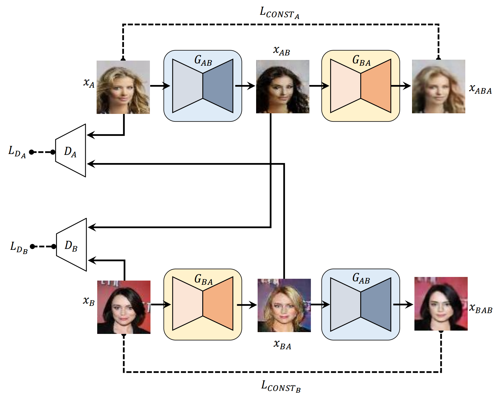
Rows from top to bottom: (1) Real image from domain A (2) Translated image from
domain A (3) Reconstructed image from domain A (4) Real image from domain B (5)
Translated image from domain B (6) Reconstructed image from domain B​

DRAGAN

On Convergence and Stability of GANs

Authors

Naveen Kodali, Jacob Abernethy, James Hays, Zsolt Kira

Abstract

We propose studying GAN training dynamics as regret minimization, which is in contrast to the popular view that there is consistent minimization of a divergence between real and generated distributions. We analyze the convergence of GAN training from this new point of view to understand why mode collapse happens. We hypothesize the existence of undesirable local equilibria in this non-convex game to be responsible for mode collapse. We observe that these local equilibria often exhibit sharp gradients of the discriminator function around some real data points. We demonstrate that these degenerate local equilibria can be avoided with a gradient penalty scheme called DRAGAN. We show that DRAGAN enables faster training, achieves improved stability with fewer mode collapses, and leads to generator networks with better modeling performance across a variety of architectures and objective functions.

[Paper] [Code]

Run Example

$ cd implementations/dragan/
$ python3 dragan.py

DualGAN

DualGAN: Unsupervised Dual Learning for Image-to-Image Translation

Authors

Zili Yi, Hao Zhang, Ping Tan, Minglun Gong

Abstract

Conditional Generative Adversarial Networks (GANs) for cross-domain image-to-image translation have made much progress recently. Depending on the task complexity, thousands to millions of labeled image pairs are needed to train a conditional GAN. However, human labeling is expensive, even impractical, and large quantities of data may not always be available. Inspired by dual learning from natural language translation, we develop a novel dual-GAN mechanism, which enables image translators to be trained from two sets of unlabeled images from two domains. In our architecture, the primal GAN learns to translate images from domain U to those in domain V, while the dual GAN learns to invert the task. The closed loop made by the primal and dual tasks allows images from either domain to be translated and then reconstructed. Hence a loss function that accounts for the reconstruction error of images can be used to train the translators. Experiments on multiple image translation tasks with unlabeled data show considerable performance gain of DualGAN over a single GAN. For some tasks, DualGAN can even achieve comparable or slightly better results than conditional GAN trained on fully labeled data.

[Paper] [Code]

Run Example

$ cd data/
$ bash download_pix2pix_dataset.sh facades
$ cd ../implementations/dualgan/
$ python3 dualgan.py --dataset_name facades

Energy-Based GAN

Energy-based Generative Adversarial Network

Authors

Junbo Zhao, Michael Mathieu, Yann LeCun

Abstract

We introduce the “Energy-based Generative Adversarial Network” model (EBGAN) which views the discriminator as an energy function that attributes low energies to the regions near the data manifold and higher energies to other regions. Similar to the probabilistic GANs, a generator is seen as being trained to produce contrastive samples with minimal energies, while the discriminator is trained to assign high energies to these generated samples. Viewing the discriminator as an energy function allows to use a wide variety of architectures and loss functionals in addition to the usual binary classifier with logistic output. Among them, we show one instantiation of EBGAN framework as using an auto-encoder architecture, with the energy being the reconstruction error, in place of the discriminator. We show that this form of EBGAN exhibits more stable behavior than regular GANs during training. We also show that a single-scale architecture can be trained to generate high-resolution images.

[Paper] [Code]

Run Example

$ cd implementations/ebgan/
$ python3 ebgan.py

Enhanced Super-Resolution GAN

ESRGAN: Enhanced Super-Resolution Generative Adversarial Networks

Authors

Xintao Wang, Ke Yu, Shixiang Wu, Jinjin Gu, Yihao Liu, Chao Dong, Chen Change Loy, Yu Qiao, Xiaoou Tang

Abstract

The Super-Resolution Generative Adversarial Network (SRGAN) is a seminal work that is capable of generating realistic textures during single image super-resolution. However, the hallucinated details are often accompanied with unpleasant artifacts. To further enhance the visual quality, we thoroughly study three key components of SRGAN – network architecture, adversarial loss and perceptual loss, and improve each of them to derive an Enhanced SRGAN (ESRGAN). In particular, we introduce the Residual-in-Residual Dense Block (RRDB) without batch normalization as the basic network building unit. Moreover, we borrow the idea from relativistic GAN to let the discriminator predict relative realness instead of the absolute value. Finally, we improve the perceptual loss by using the features before activation, which could provide stronger supervision for brightness consistency and texture recovery. Benefiting from these improvements, the proposed ESRGAN achieves consistently better visual quality with more realistic and natural textures than SRGAN and won the first place in the PIRM2018-SR Challenge. The code is available at this https URL.

[Paper] [Code]

Run Example

$ cd implementations/esrgan/
<follow steps at the top of esrgan.py>
$ python3 esrgan.py

Nearest Neighbor Upsampling | ESRGAN​

GAN

Generative Adversarial Network

Authors

Ian J. Goodfellow, Jean Pouget-Abadie, Mehdi Mirza, Bing Xu, David Warde-Farley, Sherjil Ozair, Aaron Courville, Yoshua Bengio

Abstract

We propose a new framework for estimating generative models via an adversarial process, in which we simultaneously train two models: a generative model G that captures the data distribution, and a discriminative model D that estimates the probability that a sample came from the training data rather than G. The training procedure for G is to maximize the probability of D making a mistake. This framework corresponds to a minimax two-player game. In the space of arbitrary functions G and D, a unique solution exists, with G recovering the training data distribution and D equal to 1/2 everywhere. In the case where G and D are defined by multilayer perceptrons, the entire system can be trained with backpropagation. There is no need for any Markov chains or unrolled approximate inference networks during either training or generation of samples. Experiments demonstrate the potential of the framework through qualitative and quantitative evaluation of the generated samples.

[Paper] [Code]

Run Example

$ cd implementations/gan/
$ python3 gan.py

InfoGAN

InfoGAN: Interpretable Representation Learning by Information Maximizing Generative Adversarial Nets

Authors

Xi Chen, Yan Duan, Rein Houthooft, John Schulman, Ilya Sutskever, Pieter Abbeel

Abstract

This paper describes InfoGAN, an information-theoretic extension to the Generative Adversarial Network that is able to learn disentangled representations in a completely unsupervised manner. InfoGAN is a generative adversarial network that also maximizes the mutual information between a small subset of the latent variables and the observation. We derive a lower bound to the mutual information objective that can be optimized efficiently, and show that our training procedure can be interpreted as a variation of the Wake-Sleep algorithm. Specifically, InfoGAN successfully disentangles writing styles from digit shapes on the MNIST dataset, pose from lighting of 3D rendered images, and background digits from the central digit on the SVHN dataset. It also discovers visual concepts that include hair styles, presence/absence of eyeglasses, and emotions on the CelebA face dataset. Experiments show that InfoGAN learns interpretable representations that are competitive with representations learned by existing fully supervised methods.

[Paper] [Code]

Run Example

$ cd implementations/infogan/
$ python3 infogan.py

Result of varying categorical latent variable by column.​

Result of varying continuous latent variable by row.​

Least Squares GAN

Least Squares Generative Adversarial Networks

Authors

Xudong Mao, Qing Li, Haoran Xie, Raymond Y.K. Lau, Zhen Wang, Stephen Paul Smolley

Abstract

Unsupervised learning with generative adversarial networks (GANs) has proven hugely successful. Regular GANs hypothesize the discriminator as a classifier with the sigmoid cross entropy loss function. However, we found that this loss function may lead to the vanishing gradients problem during the learning process. To overcome such a problem, we propose in this paper the Least Squares Generative Adversarial Networks (LSGANs) which adopt the least squares loss function for the discriminator. We show that minimizing the objective function of LSGAN yields minimizing the Pearson χ2 divergence. There are two benefits of LSGANs over regular GANs. First, LSGANs are able to generate higher quality images than regular GANs. Second, LSGANs perform more stable during the learning process. We evaluate LSGANs on five scene datasets and the experimental results show that the images generated by LSGANs are of better quality than the ones generated by regular GANs. We also conduct two comparison experiments between LSGANs and regular GANs to illustrate the stability of LSGANs.

[Paper] [Code]

Run Example

$ cd implementations/lsgan/
$ python3 lsgan.py

MUNIT

Multimodal Unsupervised Image-to-Image Translation

Authors

Xun Huang, Ming-Yu Liu, Serge Belongie, Jan Kautz

Abstract

Unsupervised image-to-image translation is an important and challenging problem in computer vision. Given an image in the source domain, the goal is to learn the conditional distribution of corresponding images in the target domain, without seeing any pairs of corresponding images. While this conditional distribution is inherently multimodal, existing approaches make an overly simplified assumption, modeling it as a deterministic one-to-one mapping. As a result, they fail to generate diverse outputs from a given source domain image. To address this limitation, we propose a Multimodal Unsupervised Image-to-image Translation (MUNIT) framework. We assume that the image representation can be decomposed into a content code that is domain-invariant, and a style code that captures domain-specific properties. To translate an image to another domain, we recombine its content code with a random style code sampled from the style space of the target domain. We analyze the proposed framework and establish several theoretical results. Extensive experiments with comparisons to the state-of-the-art approaches further demonstrates the advantage of the proposed framework. Moreover, our framework allows users to control the style of translation outputs by providing an example style image. Code and pretrained models are available at this https URL

[Paper] [Code]

Run Example

$ cd data/
$ bash download_pix2pix_dataset.sh edges2shoes
$ cd ../implementations/munit/
$ python3 munit.py --dataset_name edges2shoes

Results by varying the style code.​

Pix2Pix

Unpaired Image-to-Image Translation with Conditional Adversarial Networks

Authors

Phillip Isola, Jun-Yan Zhu, Tinghui Zhou, Alexei A. Efros

Abstract

We investigate conditional adversarial networks as a general-purpose solution to image-to-image translation problems. These networks not only learn the mapping from input image to output image, but also learn a loss function to train this mapping. This makes it possible to apply the same generic approach to problems that traditionally would require very different loss formulations. We demonstrate that this approach is effective at synthesizing photos from label maps, reconstructing objects from edge maps, and colorizing images, among other tasks. Indeed, since the release of the pix2pix software associated with this paper, a large number of internet users (many of them artists) have posted their own experiments with our system, further demonstrating its wide applicability and ease of adoption without the need for parameter tweaking. As a community, we no longer hand-engineer our mapping functions, and this work suggests we can achieve reasonable results without hand-engineering our loss functions either.

[Paper] [Code]

Run Example

$ cd data/
$ bash download_pix2pix_dataset.sh facades
$ cd ../implementations/pix2pix/
$ python3 pix2pix.py --dataset_name facades

Rows from top to bottom: (1) The condition for the generator (2) Generated image
based of condition (3) The true corresponding image to the condition​

PixelDA

Unsupervised Pixel-Level Domain Adaptation with Generative Adversarial Networks

Authors

Konstantinos Bousmalis, Nathan Silberman, David Dohan, Dumitru Erhan, Dilip Krishnan

Abstract

Collecting well-annotated image datasets to train modern machine learning algorithms is prohibitively expensive for many tasks. One appealing alternative is rendering synthetic data where ground-truth annotations are generated automatically. Unfortunately, models trained purely on rendered images often fail to generalize to real images. To address this shortcoming, prior work introduced unsupervised domain adaptation algorithms that attempt to map representations between the two domains or learn to extract features that are domain-invariant. In this work, we present a new approach that learns, in an unsupervised manner, a transformation in the pixel space from one domain to the other. Our generative adversarial network (GAN)-based method adapts source-domain images to appear as if drawn from the target domain. Our approach not only produces plausible samples, but also outperforms the state-of-the-art on a number of unsupervised domain adaptation scenarios by large margins. Finally, we demonstrate that the adaptation process generalizes to object classes unseen during training.

[Paper] [Code]

MNIST to MNIST-M Classification

Trains a classifier on images that have been translated from the source domain (MNIST) to the target domain (MNIST-M) using the annotations of the source domain images. The classification network is trained jointly with the generator network to optimize the generator for both providing a proper domain translation and also for preserving the semantics of the source domain image. The classification network trained on translated images is compared to the naive solution of training a classifier on MNIST and evaluating it on MNIST-M. The naive model manages a 55% classification accuracy on MNIST-M while the one trained during domain adaptation achieves a 95% classification accuracy.

$ cd implementations/pixelda/
$ python3 pixelda.py
MethodAccuracy
Naive55%
PixelDA95%

Rows from top to bottom: (1) Real images from MNIST (2) Translated images from
MNIST to MNIST-M (3) Examples of images from MNIST-M​

Relativistic GAN

The relativistic discriminator: a key element missing from standard GAN

Authors

Alexia Jolicoeur-Martineau

Abstract

In standard generative adversarial network (SGAN), the discriminator estimates the probability that the input data is real. The generator is trained to increase the probability that fake data is real. We argue that it should also simultaneously decrease the probability that real data is real because 1) this would account for a priori knowledge that half of the data in the mini-batch is fake, 2) this would be observed with divergence minimization, and 3) in optimal settings, SGAN would be equivalent to integral probability metric (IPM) GANs. We show that this property can be induced by using a relativistic discriminator which estimate the probability that the given real data is more realistic than a randomly sampled fake data. We also present a variant in which the discriminator estimate the probability that the given real data is more realistic than fake data, on average. We generalize both approaches to non-standard GAN loss functions and we refer to them respectively as Relativistic GANs (RGANs) and Relativistic average GANs (RaGANs). We show that IPM-based GANs are a subset of RGANs which use the identity function. Empirically, we observe that 1) RGANs and RaGANs are significantly more stable and generate higher quality data samples than their non-relativistic counterparts, 2) Standard RaGAN with gradient penalty generate data of better quality than WGAN-GP while only requiring a single discriminator update per generator update (reducing the time taken for reaching the state-of-the-art by 400%), and 3) RaGANs are able to generate plausible high resolutions images (256×256) from a very small sample (N=2011), while GAN and LSGAN cannot; these images are of significantly better quality than the ones generated by WGAN-GP and SGAN with spectral normalization.

[Paper] [Code]

Run Example

$ cd implementations/relativistic_gan/
$ python3 relativistic_gan.py # Relativistic Standard GAN
$ python3 relativistic_gan.py --rel_avg_gan # Relativistic Average GAN

Semi-Supervised GAN

Semi-Supervised Generative Adversarial Network

Authors

Augustus Odena

Abstract

We extend Generative Adversarial Networks (GANs) to the semi-supervised context by forcing the discriminator network to output class labels. We train a generative model G and a discriminator D on a dataset with inputs belonging to one of N classes. At training time, D is made to predict which of N+1 classes the input belongs to, where an extra class is added to correspond to the outputs of G. We show that this method can be used to create a more data-efficient classifier and that it allows for generating higher quality samples than a regular GAN.

[Paper] [Code]

Run Example

$ cd implementations/sgan/
$ python3 sgan.py

Softmax GAN

Softmax GAN

Authors

Min Lin

Abstract

Softmax GAN is a novel variant of Generative Adversarial Network (GAN). The key idea of Softmax GAN is to replace the classification loss in the original GAN with a softmax cross-entropy loss in the sample space of one single batch. In the adversarial learning of N real training samples and M generated samples, the target of discriminator training is to distribute all the probability mass to the real samples, each with probability 1M, and distribute zero probability to generated data. In the generator training phase, the target is to assign equal probability to all data points in the batch, each with probability 1M+N. While the original GAN is closely related to Noise Contrastive Estimation (NCE), we show that Softmax GAN is the Importance Sampling version of GAN. We futher demonstrate with experiments that this simple change stabilizes GAN training.

[Paper] [Code]

Run Example

$ cd implementations/softmax_gan/
$ python3 softmax_gan.py

StarGAN

StarGAN: Unified Generative Adversarial Networks for Multi-Domain Image-to-Image Translation

Authors

Yunjey Choi, Minje Choi, Munyoung Kim, Jung-Woo Ha, Sunghun Kim, Jaegul Choo

Abstract

Recent studies have shown remarkable success in image-to-image translation for two domains. However, existing approaches have limited scalability and robustness in handling more than two domains, since different models should be built independently for every pair of image domains. To address this limitation, we propose StarGAN, a novel and scalable approach that can perform image-to-image translations for multiple domains using only a single model. Such a unified model architecture of StarGAN allows simultaneous training of multiple datasets with different domains within a single network. This leads to StarGAN’s superior quality of translated images compared to existing models as well as the novel capability of flexibly translating an input image to any desired target domain. We empirically demonstrate the effectiveness of our approach on a facial attribute transfer and a facial expression synthesis tasks.

[Paper] [Code]

Run Example

$ cd implementations/stargan/
<follow steps at the top of stargan.py>
$ python3 stargan.py

Original | Black Hair | Blonde Hair | Brown Hair | Gender Flip | Aged​

Super-Resolution GAN

Photo-Realistic Single Image Super-Resolution Using a Generative Adversarial Network

Authors

Christian Ledig, Lucas Theis, Ferenc Huszar, Jose Caballero, Andrew Cunningham, Alejandro Acosta, Andrew Aitken, Alykhan Tejani, Johannes Totz, Zehan Wang, Wenzhe Shi

Abstract

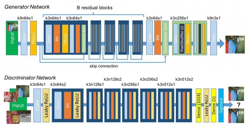
Despite the breakthroughs in accuracy and speed of single image super-resolution using faster and deeper convolutional neural networks, one central problem remains largely unsolved: how do we recover the finer texture details when we super-resolve at large upscaling factors? The behavior of optimization-based super-resolution methods is principally driven by the choice of the objective function. Recent work has largely focused on minimizing the mean squared reconstruction error. The resulting estimates have high peak signal-to-noise ratios, but they are often lacking high-frequency details and are perceptually unsatisfying in the sense that they fail to match the fidelity expected at the higher resolution. In this paper, we present SRGAN, a generative adversarial network (GAN) for image super-resolution (SR). To our knowledge, it is the first framework capable of inferring photo-realistic natural images for 4x upscaling factors. To achieve this, we propose a perceptual loss function which consists of an adversarial loss and a content loss. The adversarial loss pushes our solution to the natural image manifold using a discriminator network that is trained to differentiate between the super-resolved images and original photo-realistic images. In addition, we use a content loss motivated by perceptual similarity instead of similarity in pixel space. Our deep residual network is able to recover photo-realistic textures from heavily downsampled images on public benchmarks. An extensive mean-opinion-score (MOS) test shows hugely significant gains in perceptual quality using SRGAN. The MOS scores obtained with SRGAN are closer to those of the original high-resolution images than to those obtained with any state-of-the-art method.

[Paper] [Code]

Run Example

$ cd implementations/srgan/
<follow steps at the top of srgan.py>
$ python3 srgan.py

Nearest Neighbor Upsampling | SRGAN​

UNIT

Unsupervised Image-to-Image Translation Networks

Authors

Ming-Yu Liu, Thomas Breuel, Jan Kautz

Abstract

Unsupervised image-to-image translation aims at learning a joint distribution of images in different domains by using images from the marginal distributions in individual domains. Since there exists an infinite set of joint distributions that can arrive the given marginal distributions, one could infer nothing about the joint distribution from the marginal distributions without additional assumptions. To address the problem, we make a shared-latent space assumption and propose an unsupervised image-to-image translation framework based on Coupled GANs. We compare the proposed framework with competing approaches and present high quality image translation results on various challenging unsupervised image translation tasks, including street scene image translation, animal image translation, and face image translation. We also apply the proposed framework to domain adaptation and achieve state-of-the-art performance on benchmark datasets. Code and additional results are available in this https URL.

[Paper] [Code]

Run Example

$ cd data/
$ bash download_cyclegan_dataset.sh apple2orange
$ cd implementations/unit/
$ python3 unit.py --dataset_name apple2orange

Wasserstein GAN

Wasserstein GAN

Authors

Martin Arjovsky, Soumith Chintala, Léon Bottou

Abstract

We introduce a new algorithm named WGAN, an alternative to traditional GAN training. In this new model, we show that we can improve the stability of learning, get rid of problems like mode collapse, and provide meaningful learning curves useful for debugging and hyperparameter searches. Furthermore, we show that the corresponding optimization problem is sound, and provide extensive theoretical work highlighting the deep connections to other distances between distributions.

[Paper] [Code]

Run Example

$ cd implementations/wgan/
$ python3 wgan.py

Wasserstein GAN GP

Improved Training of Wasserstein GANs

Authors

Ishaan Gulrajani, Faruk Ahmed, Martin Arjovsky, Vincent Dumoulin, Aaron Courville

Abstract

Generative Adversarial Networks (GANs) are powerful generative models, but suffer from training instability. The recently proposed Wasserstein GAN (WGAN) makes progress toward stable training of GANs, but sometimes can still generate only low-quality samples or fail to converge. We find that these problems are often due to the use of weight clipping in WGAN to enforce a Lipschitz constraint on the critic, which can lead to undesired behavior. We propose an alternative to clipping weights: penalize the norm of gradient of the critic with respect to its input. Our proposed method performs better than standard WGAN and enables stable training of a wide variety of GAN architectures with almost no hyperparameter tuning, including 101-layer ResNets and language models over discrete data. We also achieve high quality generations on CIFAR-10 and LSUN bedrooms.

[Paper] [Code]

Run Example

$ cd implementations/wgan_gp/
$ python3 wgan_gp.py

Wasserstein GAN DIV

Wasserstein Divergence for GANs

Authors

Jiqing Wu, Zhiwu Huang, Janine Thoma, Dinesh Acharya, Luc Van Gool

Abstract

In many domains of computer vision, generative adversarial networks (GANs) have achieved great success, among which the fam- ily of Wasserstein GANs (WGANs) is considered to be state-of-the-art due to the theoretical contributions and competitive qualitative performance. However, it is very challenging to approximate the k-Lipschitz constraint required by the Wasserstein-1 metric (W-met). In this paper, we propose a novel Wasserstein divergence (W-div), which is a relaxed version of W-met and does not require the k-Lipschitz constraint.As a concrete application, we introduce a Wasserstein divergence objective for GANs (WGAN-div), which can faithfully approximate W-div through optimization. Under various settings, including progressive growing training, we demonstrate the stability of the proposed WGAN-div owing to its theoretical and practical advantages over WGANs. Also, we study the quantitative and visual performance of WGAN-div on standard image synthesis benchmarks, showing the superior performance of WGAN-div compared to the state-of-the-art methods.

[Paper] [Code]

Run Example

$ cd implementations/wgan_div/
$ python3 wgan_div.py

命名张量

张量命名是一个非常有用的方法,这样可以方便地使用维度的名字来做索引或其他操作,大大提高了可读性、易用性,防止出错。

命名的对象是张量的维度:

NCHW = [‘N’, ‘C’, ‘H’, ‘W’]
#张量命名
images = torch.randn(32, 3, 56, 56, names=NCHW)
images.sum('C')
images.select('C', index=0)
# 也可以这么设置
tensor = torch.rand(3,4,1,2,names=('C', 'N', 'H', 'W'))
# 使用align_to可以对维度方便地排序
tensor = tensor.align_to('N', 'C', 'H', 'W')

命名张量允许用户为张量维度指定明确的名称。在大多数情况下,采用维度参数的操作将接受维度名称,从而无需按位置跟踪维度。此外,命名张量使用名称来自动检查 API 在运行时是否被正确使用,从而提供额外的安全性。名称还可用于重新排列维度,例如,支持“按名称广播”而不是“按位置广播”。

使用方法:对于任意张量,采用一个 names 参数,参数值是一个字符类型列表or元组,值表示维度名称,将名称与每个维度相关联。

>>> torch.zeros(2, 3, names=('N', 'C'))
tensor([[0., 0., 0.],
        [0., 0., 0.]], names=('N', 'C'))


<!-- wp:preformatted -->
<pre id="codecell0" class="wp-block-preformatted">>>> <strong>torch.zeros(</strong>2<strong>,</strong> 3<strong>,</strong> <strong>names=(</strong>'N'<strong>,</strong> 'C'<strong>))</strong>
tensor([[0., 0., 0.],
        [0., 0., 0.]], names=('N', 'C'))


#获得维度的名称为i的tensor
tensor.names[i]#获得为维度的名称i的tensor

以下函数支持命名张量:

使用tensor.names访问张量的维度名称和 tensor.rename()重命名命名:

>>> imgs = torch.randn(1, 2, 2, 3 , names=('N', 'C', 'H', 'W'))
>>> imgs.names
('N', 'C', 'H', 'W')

>>> renamed_imgs = imgs.rename(H='height', W='width')
>>> renamed_imgs.names
('N', 'C', 'height', 'width)

命名张量可以与未命名张量共存;命名张量是 的实例 torch.Tensor。未命名张量具有命名None维度。命名张量不需要命名所有维度。

>>> imgs = torch.randn(1, 2, 2, 3 , names=(None, 'C', 'H', 'W'))
>>> imgs.names
(None, 'C', 'H', 'W')

名称传播语义

命名张量使用名称来自动检查 API 在运行时是否被正确调用。这发生在一个名为name inference的过程中。更正式地说,名称推断包括以下两个步骤:

  • 检查名称:操作员可以在运行时执行自动检查,以检查某些维度名称是否必须匹配。
  • 传播名称:名称推断将名称传播到输出张量。

所有支持命名张量的操作都会传播名称。

>>> x = torch.randn(3, 3, names=('N', 'C'))
>>> x.abs().names
('N', 'C')

官方文档地址: https://pytorch.org/docs/stable/named_tensor.html

PyTorch常用代码段合集

挺有用的,保留下来,撸代码的时候参考备用。

作者丨Jack Stark@知乎

来源丨https://zhuanlan.zhihu.com/p/104019160

本文是PyTorch常用代码段合集,涵盖基本配置、张量处理、模型定义与操作、数据处理、模型训练与测试等5个方面,还给出了多个值得注意的Tips,内容非常全面。

PyTorch最好的资料是官方文档。本文是PyTorch常用代码段,在参考资料[1](张皓:PyTorch Cookbook)的基础上做了一些修补,方便使用时查阅。

1. 基本配置

导入包和版本查询

import torch
import torch.nn as nn
import torchvision
print(torch.__version__)
print(torch.version.cuda)
print(torch.backends.cudnn.version())
print(torch.cuda.get_device_name(0))

可复现性

在硬件设备(CPU、GPU)不同时,完全的可复现性无法保证,即使随机种子相同。但是,在同一个设备上,应该保证可复现性。具体做法是,在程序开始的时候固定torch的随机种子,同时也把numpy的随机种子固定。

np.random.seed(0)
torch.manual_seed(0)
torch.cuda.manual_seed_all(0)
torch.backends.cudnn.deterministic = True
torch.backends.cudnn.benchmark = False

显卡设置

如果只需要一张显卡

# Device configuration
device = torch.device('cuda' if torch.cuda.is_available() else 'cpu')

如果需要指定多张显卡,比如0,1号显卡。

import os
os.environ['CUDA_VISIBLE_DEVICES'] = '0,1'

也可以在命令行运行代码时设置显卡:

CUDA_VISIBLE_DEVICES=0,1 python train.py

清除显存

torch.cuda.empty_cache()

也可以使用在命令行重置GPU的指令

nvidia-smi --gpu-reset -i [gpu_id]

2. 张量(Tensor)处理

张量的数据类型

PyTorch有9种CPU张量类型和9种GPU张量类型。

张量基本信息

tensor = torch.randn(3,4,5)
print(tensor.type())  # 数据类型
print(tensor.size())  # 张量的shape,是个元组
print(tensor.dim())   # 维度的数量

命名张量

张量命名是一个非常有用的方法,这样可以方便地使用维度的名字来做索引或其他操作,大大提高了可读性、易用性,防止出错。、

# 在PyTorch 1.3之前,需要使用注释
# Tensor[N, C, H, W]
images = torch.randn(32, 3, 56, 56)
images.sum(dim=1)
images.select(dim=1, index=0)

# PyTorch 1.3之后
NCHW = [‘N’, ‘C’, ‘H’, ‘W’]
images = torch.randn(32, 3, 56, 56, names=NCHW)
images.sum('C')
images.select('C', index=0)
# 也可以这么设置
tensor = torch.rand(3,4,1,2,names=('C', 'N', 'H', 'W'))
# 使用align_to可以对维度方便地排序
tensor = tensor.align_to('N', 'C', 'H', 'W')

数据类型转换


# 设置默认类型,pytorch中的FloatTensor远远快于DoubleTensor
torch.set_default_tensor_type(torch.FloatTensor)

# 类型转换
tensor = tensor.cuda()
tensor = tensor.cpu()
tensor = tensor.float()
tensor = tensor.long()

torch.Tensor与np.ndarray转换

除了CharTensor,其他所有CPU上的张量都支持转换为numpy格式然后再转换回来。

ndarray = tensor.cpu().numpy()
tensor = torch.from_numpy(ndarray).float()
tensor = torch.from_numpy(ndarray.copy()).float() # If ndarray has negative stride.

Torch.tensor与PIL.Image转换

# pytorch中的张量默认采用[N, C, H, W]的顺序,并且数据范围在[0,1],需要进行转置和规范化
# torch.Tensor -> PIL.Image
image = PIL.Image.fromarray(torch.clamp(tensor*255, min=0, max=255).byte().permute(1,2,0).cpu().numpy())
image = torchvision.transforms.functional.to_pil_image(tensor)  # Equivalently way

# PIL.Image -> torch.Tensor
path = r'./figure.jpg'
tensor = torch.from_numpy(np.asarray(PIL.Image.open(path))).permute(2,0,1).float() / 255
tensor = torchvision.transforms.functional.to_tensor(PIL.Image.open(path)) # Equivalently way

np.ndarray与PIL.Image的转换

image = PIL.Image.fromarray(ndarray.astype(np.uint8))

ndarray = np.asarray(PIL.Image.open(path))

从只包含一个元素的张量中提取值


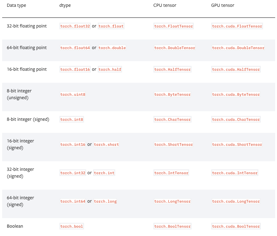
value = torch.rand(1).item()

item() → number  将单个元素的tensor数值转换为普通的python数值。
Returns the value of this tensor as a standard Python number. This only works for tensors with one element. For other cases, see tolist().

This operation is not differentiable.

Example:

>>> x = torch.tensor([1.0])
>>> x.item()
1.0

torch向量转python list :tolist()

tolist() -> list or number

Returns the tensor as a (nested) list. For scalars, a standard Python number is returned, just like with item(). Tensors are automatically moved to the CPU first if necessary.

This operation is not differentiable.

Examples:

>>> a = torch.randn(2, 2)
>>> a.tolist()
[[0.012766935862600803, 0.5415473580360413],
 [-0.08909505605697632, 0.7729271650314331]]
>>> a[0,0].tolist()
0.012766935862600803

张量形变

# 在将卷积层输入全连接层的情况下通常需要对张量做形变处理,
# 相比torch.view,torch.reshape可以自动处理输入张量不连续的情况。
tensor = torch.rand(2,3,4)
shape = (6, 4)
tensor = torch.reshape(tensor, shape)

打乱顺序

tensor = tensor[torch.randperm(tensor.size(0))]  # 打乱第一个维度

水平翻转

# pytorch不支持tensor[::-1]这样的负步长操作,水平翻转可以通过张量索引实现
# 假设张量的维度为[N, D, H, W].
tensor = tensor[:,:,:,torch.arange(tensor.size(3) - 1, -1, -1).long()]

复制张量

# Operation                 |  New/Shared memory | Still in computation graph |
tensor.clone()            # |        New         |          Yes               |
tensor.detach()           # |      Shared        |          No                |
tensor.detach.clone()()   # |        New         |          No                |

张量拼接


'''
注意torch.cat和torch.stack的区别在于torch.cat沿着给定的维度拼接,
而torch.stack会新增一维。例如当参数是3个10x5的张量,torch.cat的结果是30x5的张量,
而torch.stack的结果是3x10x5的张量。
'''
tensor = torch.cat(list_of_tensors, dim=0)
tensor = torch.stack(list_of_tensors, dim=0)

将整数标签转为one-hot编码


# pytorch的标记默认从0开始
tensor = torch.tensor([0, 2, 1, 3])
N = tensor.size(0)
num_classes = 4
one_hot = torch.zeros(N, num_classes).long()
one_hot.scatter_(dim=1, index=torch.unsqueeze(tensor, dim=1), src=torch.ones(N, num_classes).long())

得到非零元素

torch.nonzero(tensor)               # index of non-zero elements
torch.nonzero(tensor==0)            # index of zero elements
torch.nonzero(tensor).size(0)       # number of non-zero elements
torch.nonzero(tensor == 0).size(0)  # number of zero elements

判断两个张量相等
torch.allclose(tensor1, tensor2)  # float tensor
torch.equal(tensor1, tensor2)     # int tensor
张量扩展
# Expand tensor of shape 64*512 to shape 64*512*7*7.
tensor = torch.rand(64,512)
torch.reshape(tensor, (64, 512, 1, 1)).expand(64, 512, 7, 7)
矩阵乘法
# Matrix multiplcation: (m*n) * (n*p) * -> (m*p).
result = torch.mm(tensor1, tensor2)

# Batch matrix multiplication: (b*m*n) * (b*n*p) -> (b*m*p)
result = torch.bmm(tensor1, tensor2)

# Element-wise multiplication.
result = tensor1 * tensor2

计算两组数据之间的两两欧式距离
利用broadcast机制
dist = torch.sqrt(torch.sum((X1[:,None,:] - X2) ** 2, dim=2))

3. 模型定义和操作

一个简单两层卷积网络的示例


# convolutional neural network (2 convolutional layers)
class ConvNet(nn.Module):
    def __init__(self, num_classes=10):
        super(ConvNet, self).__init__()
        self.layer1 = nn.Sequential(
            nn.Conv2d(1, 16, kernel_size=5, stride=1, padding=2),
            nn.BatchNorm2d(16),
            nn.ReLU(),
            nn.MaxPool2d(kernel_size=2, stride=2))
        self.layer2 = nn.Sequential(
            nn.Conv2d(16, 32, kernel_size=5, stride=1, padding=2),
            nn.BatchNorm2d(32),
            nn.ReLU(),
            nn.MaxPool2d(kernel_size=2, stride=2))
        self.fc = nn.Linear(7*7*32, num_classes)

    def forward(self, x):
        out = self.layer1(x)
        out = self.layer2(out)
        out = out.reshape(out.size(0), -1)
        out = self.fc(out)
        return out


model = ConvNet(num_classes).to(device)

卷积层的计算和展示可以用这个网站辅助。

双线性汇合(bilinear pooling)

X = torch.reshape(N, D, H * W)                        # Assume X has shape N*D*H*W
X = torch.bmm(X, torch.transpose(X, 1, 2)) / (H * W)  # Bilinear pooling
assert X.size() == (N, D, D)
X = torch.reshape(X, (N, D * D))
X = torch.sign(X) * torch.sqrt(torch.abs(X) + 1e-5)   # Signed-sqrt normalization
X = torch.nn.functional.normalize(X)                  # L2 normalization

多卡同步 BN(Batch normalization)

当使用 torch.nn.DataParallel 将代码运行在多张 GPU 卡上时,PyTorch 的 BN 层默认操作是各卡上数据独立地计算均值和标准差,同步 BN 使用所有卡上的数据一起计算 BN 层的均值和标准差,缓解了当批量大小(batch size)比较小时对均值和标准差估计不准的情况,是在目标检测等任务中一个有效的提升性能的技巧。

sync_bn = torch.nn.SyncBatchNorm(num_features, eps=1e-05, momentum=0.1, affine=True, 
                                 track_running_stats=True)

将已有网络的所有BN层改为同步BN层

def convertBNtoSyncBN(module, process_group=None):
    '''Recursively replace all BN layers to SyncBN layer.

    Args:
        module[torch.nn.Module]. Network
    '''
    if isinstance(module, torch.nn.modules.batchnorm._BatchNorm):
        sync_bn = torch.nn.SyncBatchNorm(module.num_features, module.eps, module.momentum, 
                                         module.affine, module.track_running_stats, process_group)
        sync_bn.running_mean = module.running_mean
        sync_bn.running_var = module.running_var
        if module.affine:
            sync_bn.weight = module.weight.clone().detach()
            sync_bn.bias = module.bias.clone().detach()
        return sync_bn
    else:
        for name, child_module in module.named_children():
            setattr(module, name) = convert_syncbn_model(child_module, process_group=process_group))
        return module

类似 BN 滑动平均

如果要实现类似 BN 滑动平均的操作,在 forward 函数中要使用原地(inplace)操作给滑动平均赋值。

class BN(torch.nn.Module)
    def __init__(self):
        ...
        self.register_buffer('running_mean', torch.zeros(num_features))

    def forward(self, X):
        ...
        self.running_mean += momentum * (current - self.running_mean)
计算模型整体参数量

num_parameters = sum(torch.numel(parameter) for parameter in model.parameters())

查看网络中的参数

可以通过model.state_dict()或者model.named_parameters()函数查看现在的全部可训练参数(包括通过继承得到的父类中的参数)
params = list(model.named_parameters())
(name, param) = params[28]
print(name)
print(param.grad)
print('-------------------------------------------------')
(name2, param2) = params[29]
print(name2)
print(param2.grad)
print('----------------------------------------------------')
(name1, param1) = params[30]
print(name1)
print(param1.grad)

模型可视化(使用pytorchviz)

szagoruyko/pytorchvizgithub.com
类似 Keras 的 model.summary() 输出模型信息,使用pytorch-summary
sksq96/pytorch-summarygithub.com

模型权重初始化
注意 model.modules() 和 model.children() 的区别:model.modules() 会迭代地遍历模型的所有子层,而 model.children() 只会遍历模型下的一层。

# Common practise for initialization.
for layer in model.modules():
    if isinstance(layer, torch.nn.Conv2d):
        torch.nn.init.kaiming_normal_(layer.weight, mode='fan_out',
                                      nonlinearity='relu')
        if layer.bias is not None:
            torch.nn.init.constant_(layer.bias, val=0.0)
    elif isinstance(layer, torch.nn.BatchNorm2d):
        torch.nn.init.constant_(layer.weight, val=1.0)
        torch.nn.init.constant_(layer.bias, val=0.0)
    elif isinstance(layer, torch.nn.Linear):
        torch.nn.init.xavier_normal_(layer.weight)
        if layer.bias is not None:
            torch.nn.init.constant_(layer.bias, val=0.0)

# Initialization with given tensor.
layer.weight = torch.nn.Parameter(tensor)

提取模型中的某一层
modules()会返回模型中所有模块的迭代器,它能够访问到最内层,比如self.layer1.conv1这个模块,还有一个与它们相对应的是name_children()属性以及named_modules(),这两个不仅会返回模块的迭代器,还会返回网络层的名字。
# 取模型中的前两层
new_model = nn.Sequential(*list(model.children())[:2] 
# 如果希望提取出模型中的所有卷积层,可以像下面这样操作:
for layer in model.named_modules():
    if isinstance(layer[1],nn.Conv2d):
         conv_model.add_module(layer[0],layer[1])


部分层使用预训练模型
注意如果保存的模型是 torch.nn.DataParallel,则当前的模型也需要是
model.load_state_dict(torch.load('model.pth'), strict=False)
将在 GPU 保存的模型加载到 CPU
model.load_state_dict(torch.load('model.pth', map_location='cpu'))

导入另一个模型的相同部分到新的模型
模型导入参数时,如果两个模型结构不一致,则直接导入参数会报错。用下面方法可以把另一个模型的相同的部分导入到新的模型中。
# model_new代表新的模型
# model_saved代表其他模型,比如用torch.load导入的已保存的模型
model_new_dict = model_new.state_dict()
model_common_dict = {k:v for k, v in model_saved.items() if k in model_new_dict.keys()}
model_new_dict.update(model_common_dict)
model_new.load_state_dict(model_new_dict)

4. 数据处理

计算数据集的均值和标准差
import os
import cv2
import numpy as np
from torch.utils.data import Dataset
from PIL import Image


def compute_mean_and_std(dataset):
    # 输入PyTorch的dataset,输出均值和标准差
    mean_r = 0
    mean_g = 0
    mean_b = 0

    for img, _ in dataset:
        img = np.asarray(img) # change PIL Image to numpy array
        mean_b += np.mean(img[:, :, 0])
        mean_g += np.mean(img[:, :, 1])
        mean_r += np.mean(img[:, :, 2])

    mean_b /= len(dataset)
    mean_g /= len(dataset)
    mean_r /= len(dataset)

    diff_r = 0
    diff_g = 0
    diff_b = 0

    N = 0

    for img, _ in dataset:
        img = np.asarray(img)

        diff_b += np.sum(np.power(img[:, :, 0] - mean_b, 2))
        diff_g += np.sum(np.power(img[:, :, 1] - mean_g, 2))
        diff_r += np.sum(np.power(img[:, :, 2] - mean_r, 2))

        N += np.prod(img[:, :, 0].shape)

    std_b = np.sqrt(diff_b / N)
    std_g = np.sqrt(diff_g / N)
    std_r = np.sqrt(diff_r / N)

    mean = (mean_b.item() / 255.0, mean_g.item() / 255.0, mean_r.item() / 255.0)
    std = (std_b.item() / 255.0, std_g.item() / 255.0, std_r.item() / 255.0)
    return mean, std


得到视频数据基本信息
import cv2
video = cv2.VideoCapture(mp4_path)
height = int(video.get(cv2.CAP_PROP_FRAME_HEIGHT))
width = int(video.get(cv2.CAP_PROP_FRAME_WIDTH))
num_frames = int(video.get(cv2.CAP_PROP_FRAME_COUNT))
fps = int(video.get(cv2.CAP_PROP_FPS))
video.release()
TSN 每段(segment)采样一帧视频
K = self._num_segments
if is_train:
    if num_frames > K:
        # Random index for each segment.
        frame_indices = torch.randint(
            high=num_frames // K, size=(K,), dtype=torch.long)
        frame_indices += num_frames // K * torch.arange(K)
    else:
        frame_indices = torch.randint(
            high=num_frames, size=(K - num_frames,), dtype=torch.long)
        frame_indices = torch.sort(torch.cat((
            torch.arange(num_frames), frame_indices)))[0]
else:
    if num_frames > K:
        # Middle index for each segment.
        frame_indices = num_frames / K // 2
        frame_indices += num_frames // K * torch.arange(K)
    else:
        frame_indices = torch.sort(torch.cat((                              
            torch.arange(num_frames), torch.arange(K - num_frames))))[0]
assert frame_indices.size() == (K,)
return [frame_indices[i] for i in range(K)]


常用训练和验证数据预处理
其中 ToTensor 操作会将 PIL.Image 或形状为 H×W×D,数值范围为 [0, 255] 的 np.ndarray 转换为形状为 D×H×W,数值范围为 [0.0, 1.0] 的 torch.Tensor。
train_transform = torchvision.transforms.Compose([
    torchvision.transforms.RandomResizedCrop(size=224,
                                             scale=(0.08, 1.0)),
    torchvision.transforms.RandomHorizontalFlip(),
    torchvision.transforms.ToTensor(),
    torchvision.transforms.Normalize(mean=(0.485, 0.456, 0.406),
                                     std=(0.229, 0.224, 0.225)),
 ])
 val_transform = torchvision.transforms.Compose([
    torchvision.transforms.Resize(256),
    torchvision.transforms.CenterCrop(224),
    torchvision.transforms.ToTensor(),
    torchvision.transforms.Normalize(mean=(0.485, 0.456, 0.406),
                                     std=(0.229, 0.224, 0.225)),
])

5. 模型训练和测试

分类模型训练代码
# Loss and optimizer
criterion = nn.CrossEntropyLoss()
optimizer = torch.optim.Adam(model.parameters(), lr=learning_rate)

# Train the model
total_step = len(train_loader)
for epoch in range(num_epochs):
    for i ,(images, labels) in enumerate(train_loader):
        images = images.to(device)
        labels = labels.to(device)

        # Forward pass
        outputs = model(images)
        loss = criterion(outputs, labels)

        # Backward and optimizer
        optimizer.zero_grad()
        loss.backward()
        optimizer.step()

        if (i+1) % 100 == 0:
            print('Epoch: [{}/{}], Step: [{}/{}], Loss: {}'
                  .format(epoch+1, num_epochs, i+1, total_step, loss.item()))


分类模型测试代码
# Test the model
model.eval()  # eval mode(batch norm uses moving mean/variance 
              #instead of mini-batch mean/variance)
with torch.no_grad():
    correct = 0
    total = 0
    for images, labels in test_loader:
        images = images.to(device)
        labels = labels.to(device)
        outputs = model(images)
        _, predicted = torch.max(outputs.data, 1)
        total += labels.size(0)
        correct += (predicted == labels).sum().item()

    print('Test accuracy of the model on the 10000 test images: {} %'
          .format(100 * correct / total))


自定义loss
继承torch.nn.Module类写自己的loss。
class MyLoss(torch.nn.Moudle):
    def __init__(self):
        super(MyLoss, self).__init__()

    def forward(self, x, y):
        loss = torch.mean((x - y) ** 2)
        return loss


标签平滑(label smoothing)
写一个label_smoothing.py的文件,然后在训练代码里引用,用LSR代替交叉熵损失即可。label_smoothing.py内容如下:
import torch
import torch.nn as nn


class LSR(nn.Module):

    def __init__(self, e=0.1, reduction='mean'):
        super().__init__()

        self.log_softmax = nn.LogSoftmax(dim=1)
        self.e = e
        self.reduction = reduction

    def _one_hot(self, labels, classes, value=1):
        """
            Convert labels to one hot vectors

        Args:
            labels: torch tensor in format [label1, label2, label3, ...]
            classes: int, number of classes
            value: label value in one hot vector, default to 1

        Returns:
            return one hot format labels in shape [batchsize, classes]
        """

        one_hot = torch.zeros(labels.size(0), classes)

        #labels and value_added  size must match
        labels = labels.view(labels.size(0), -1)
        value_added = torch.Tensor(labels.size(0), 1).fill_(value)

        value_added = value_added.to(labels.device)
        one_hot = one_hot.to(labels.device)

        one_hot.scatter_add_(1, labels, value_added)

        return one_hot

    def _smooth_label(self, target, length, smooth_factor):
        """convert targets to one-hot format, and smooth
        them.
        Args:
            target: target in form with [label1, label2, label_batchsize]
            length: length of one-hot format(number of classes)
            smooth_factor: smooth factor for label smooth

        Returns:
            smoothed labels in one hot format
        """
        one_hot = self._one_hot(target, length, value=1 - smooth_factor)
        one_hot += smooth_factor / (length - 1)

        return one_hot.to(target.device)

    def forward(self, x, target):

        if x.size(0) != target.size(0):
            raise ValueError('Expected input batchsize ({}) to match target batch_size({})'
                    .format(x.size(0), target.size(0)))

        if x.dim() < 2:
            raise ValueError('Expected input tensor to have least 2 dimensions(got {})'
                    .format(x.size(0)))

        if x.dim() != 2:
            raise ValueError('Only 2 dimension tensor are implemented, (got {})'
                    .format(x.size()))


        smoothed_target = self._smooth_label(target, x.size(1), self.e)
        x = self.log_softmax(x)
        loss = torch.sum(- x * smoothed_target, dim=1)

        if self.reduction == 'none':
            return loss

        elif self.reduction == 'sum':
            return torch.sum(loss)

        elif self.reduction == 'mean':
            return torch.mean(loss)

        else:
            raise ValueError('unrecognized option, expect reduction to be one of none, mean, sum')
或者直接在训练文件里做label smoothing
for images, labels in train_loader:
    images, labels = images.cuda(), labels.cuda()
    N = labels.size(0)
    # C is the number of classes.
    smoothed_labels = torch.full(size=(N, C), fill_value=0.1 / (C - 1)).cuda()
    smoothed_labels.scatter_(dim=1, index=torch.unsqueeze(labels, dim=1), value=0.9)

    score = model(images)
    log_prob = torch.nn.functional.log_softmax(score, dim=1)
    loss = -torch.sum(log_prob * smoothed_labels) / N
    optimizer.zero_grad()
    loss.backward()
    optimizer.step()


Mixup训练
beta_distribution = torch.distributions.beta.Beta(alpha, alpha)
for images, labels in train_loader:
    images, labels = images.cuda(), labels.cuda()

    # Mixup images and labels.
    lambda_ = beta_distribution.sample([]).item()
    index = torch.randperm(images.size(0)).cuda()
    mixed_images = lambda_ * images + (1 - lambda_) * images[index, :]
    label_a, label_b = labels, labels[index]

    # Mixup loss.
    scores = model(mixed_images)
    loss = (lambda_ * loss_function(scores, label_a)
            + (1 - lambda_) * loss_function(scores, label_b))
    optimizer.zero_grad()
    loss.backward()
    optimizer.step()


L1 正则化
l1_regularization = torch.nn.L1Loss(reduction='sum')
loss = ...  # Standard cross-entropy loss
for param in model.parameters():
    loss += torch.sum(torch.abs(param))
loss.backward()


不对偏置项进行权重衰减(weight decay)
pytorch里的weight decay相当于l2正则
bias_list = (param for name, param in model.named_parameters() if name[-4:] == 'bias')
others_list = (param for name, param in model.named_parameters() if name[-4:] != 'bias')
parameters = [{'parameters': bias_list, 'weight_decay': 0},                
              {'parameters': others_list}]
optimizer = torch.optim.SGD(parameters, lr=1e-2, momentum=0.9, weight_decay=1e-4)


梯度裁剪(gradient clipping)
torch.nn.utils.clip_grad_norm_(model.parameters(), max_norm=20)


得到当前学习率
# If there is one global learning rate (which is the common case).
lr = next(iter(optimizer.param_groups))['lr']

# If there are multiple learning rates for different layers.
all_lr = []
for param_group in optimizer.param_groups:
    all_lr.append(param_group['lr'])
另一种方法,在一个batch训练代码里,当前的lr是optimizer.param_groups[0]['lr']


学习率衰减
# Reduce learning rate when validation accuarcy plateau.
scheduler = torch.optim.lr_scheduler.ReduceLROnPlateau(optimizer, mode='max', patience=5, verbose=True)
for t in range(0, 80):
    train(...)
    val(...)
    scheduler.step(val_acc)

# Cosine annealing learning rate.
scheduler = torch.optim.lr_scheduler.CosineAnnealingLR(optimizer, T_max=80)
# Reduce learning rate by 10 at given epochs.
scheduler = torch.optim.lr_scheduler.MultiStepLR(optimizer, milestones=[50, 70], gamma=0.1)
for t in range(0, 80):
    scheduler.step()    
    train(...)
    val(...)

# Learning rate warmup by 10 epochs.
scheduler = torch.optim.lr_scheduler.LambdaLR(optimizer, lr_lambda=lambda t: t / 10)
for t in range(0, 10):
    scheduler.step()
    train(...)
    val(...)


优化器链式更新
从1.4版本开始,torch.optim.lr_scheduler 支持链式更新(chaining),即用户可以定义两个 schedulers,并交替在训练中使用。
import torch
from torch.optim import SGD
from torch.optim.lr_scheduler import ExponentialLR, StepLR
model = [torch.nn.Parameter(torch.randn(2, 2, requires_grad=True))]
optimizer = SGD(model, 0.1)
scheduler1 = ExponentialLR(optimizer, gamma=0.9)
scheduler2 = StepLR(optimizer, step_size=3, gamma=0.1)
for epoch in range(4):
    print(epoch, scheduler2.get_last_lr()[0])
    optimizer.step()
    scheduler1.step()
    scheduler2.step()


模型训练可视化
PyTorch可以使用tensorboard来可视化训练过程。
安装和运行TensorBoard。
pip install tensorboard
tensorboard --logdir=runs
使用SummaryWriter类来收集和可视化相应的数据,放了方便查看,可以使用不同的文件夹,比如'Loss/train'和'Loss/test'。
from torch.utils.tensorboard import SummaryWriter
import numpy as np

writer = SummaryWriter()

for n_iter in range(100):
    writer.add_scalar('Loss/train', np.random.random(), n_iter)
    writer.add_scalar('Loss/test', np.random.random(), n_iter)
    writer.add_scalar('Accuracy/train', np.random.random(), n_iter)
    writer.add_scalar('Accuracy/test', np.random.random(), n_iter)


保存与加载断点
注意为了能够恢复训练,我们需要同时保存模型和优化器的状态,以及当前的训练轮数。
start_epoch = 0
# Load checkpoint.
if resume: # resume为参数,第一次训练时设为0,中断再训练时设为1
    model_path = os.path.join('model', 'best_checkpoint.pth.tar')
    assert os.path.isfile(model_path)
    checkpoint = torch.load(model_path)
    best_acc = checkpoint['best_acc']
    start_epoch = checkpoint['epoch']
    model.load_state_dict(checkpoint['model'])
    optimizer.load_state_dict(checkpoint['optimizer'])
    print('Load checkpoint at epoch {}.'.format(start_epoch))
    print('Best accuracy so far {}.'.format(best_acc))

# Train the model
for epoch in range(start_epoch, num_epochs): 
    ... 

    # Test the model
    ...

    # save checkpoint
    is_best = current_acc > best_acc
    best_acc = max(current_acc, best_acc)
    checkpoint = {
        'best_acc': best_acc,
        'epoch': epoch + 1,
        'model': model.state_dict(),
        'optimizer': optimizer.state_dict(),
    }
    model_path = os.path.join('model', 'checkpoint.pth.tar')
    best_model_path = os.path.join('model', 'best_checkpoint.pth.tar')
    torch.save(checkpoint, model_path)
    if is_best:
        shutil.copy(model_path, best_model_path)


提取 ImageNet 预训练模型某层的卷积特征
# VGG-16 relu5-3 feature.
model = torchvision.models.vgg16(pretrained=True).features[:-1]
# VGG-16 pool5 feature.
model = torchvision.models.vgg16(pretrained=True).features
# VGG-16 fc7 feature.
model = torchvision.models.vgg16(pretrained=True)
model.classifier = torch.nn.Sequential(*list(model.classifier.children())[:-3])
# ResNet GAP feature.
model = torchvision.models.resnet18(pretrained=True)
model = torch.nn.Sequential(collections.OrderedDict(
    list(model.named_children())[:-1]))

with torch.no_grad():
    model.eval()
    conv_representation = model(image)


提取 ImageNet 预训练模型多层的卷积特征
class FeatureExtractor(torch.nn.Module):
    """Helper class to extract several convolution features from the given
    pre-trained model.

    Attributes:
        _model, torch.nn.Module.
        _layers_to_extract, list<str> or set<str>

    Example:
        >>> model = torchvision.models.resnet152(pretrained=True)
        >>> model = torch.nn.Sequential(collections.OrderedDict(
                list(model.named_children())[:-1]))
        >>> conv_representation = FeatureExtractor(
                pretrained_model=model,
                layers_to_extract={'layer1', 'layer2', 'layer3', 'layer4'})(image)
    """
    def __init__(self, pretrained_model, layers_to_extract):
        torch.nn.Module.__init__(self)
        self._model = pretrained_model
        self._model.eval()
        self._layers_to_extract = set(layers_to_extract)

    def forward(self, x):
        with torch.no_grad():
            conv_representation = []
            for name, layer in self._model.named_children():
                x = layer(x)
                if name in self._layers_to_extract:
                    conv_representation.append(x)
            return conv_representation


微调全连接层
model = torchvision.models.resnet18(pretrained=True)
for param in model.parameters():
    param.requires_grad = False
model.fc = nn.Linear(512, 100)  # Replace the last fc layer
optimizer = torch.optim.SGD(model.fc.parameters(), lr=1e-2, momentum=0.9, weight_decay=1e-4)


以较大学习率微调全连接层,较小学习率微调卷积层
model = torchvision.models.resnet18(pretrained=True)
finetuned_parameters = list(map(id, model.fc.parameters()))
conv_parameters = (p for p in model.parameters() if id(p) not in finetuned_parameters)
parameters = [{'params': conv_parameters, 'lr': 1e-3}, 
              {'params': model.fc.parameters()}]
optimizer = torch.optim.SGD(parameters, lr=1e-2, momentum=0.9, weight_decay=1e-4)

6. 其他注意事项


不要使用太大的线性层。因为nn.Linear(m,n)使用的是的内存,线性层太大很容易超出现有显存。

不要在太长的序列上使用RNN。因为RNN反向传播使用的是BPTT算法,其需要的内存和输入序列的长度呈线性关系。

model(x) 前用 model.train() 和 model.eval() 切换网络状态。
不需要计算梯度的代码块用 with torch.no_grad() 包含起来。

model.eval() 和 torch.no_grad() 的区别在于,model.eval() 是将网络切换为测试状态,例如 BN 和dropout在训练和测试阶段使用不同的计算方法。torch.no_grad() 是关闭 PyTorch 张量的自动求导机制,以减少存储使用和加速计算,得到的结果无法进行 loss.backward()。

model.zero_grad()会把整个模型的参数的梯度都归零, 而optimizer.zero_grad()只会把传入其中的参数的梯度归零.

torch.nn.CrossEntropyLoss 的输入不需要经过 Softmax。torch.nn.CrossEntropyLoss 等价于 torch.nn.functional.log_softmax + torch.nn.NLLLoss。

loss.backward() 前用 optimizer.zero_grad() 清除累积梯度。

torch.utils.data.DataLoader 中尽量设置 pin_memory=True,对特别小的数据集如 MNIST 设置 pin_memory=False 反而更快一些。num_workers 的设置需要在实验中找到最快的取值。

用 del 及时删除不用的中间变量,节约 GPU 存储。
使用 inplace 操作可节约 GPU 存储,如x = torch.nn.functional.relu(x, inplace=True)
减少 CPU 和 GPU 之间的数据传输。例如如果你想知道一个 epoch 中每个 mini-batch 的 loss 和准确率,先将它们累积在 GPU 中等一个 epoch 结束之后一起传输回 CPU 会比每个 mini-batch 都进行一次 GPU 到 CPU 的传输更快。

使用半精度浮点数 half() 会有一定的速度提升,具体效率依赖于 GPU 型号。需要小心数值精度过低带来的稳定性问题。
时常使用 assert tensor.size() == (N, D, H, W) 作为调试手段,确保张量维度和你设想中一致。

除了标记 y 外,尽量少使用一维张量,使用 n*1 的二维张量代替,可以避免一些意想不到的一维张量计算结果。

统计代码各部分耗时

with torch.autograd.profiler.profile(enabled=True, use_cuda=False) as profile:    ...print(profile)# 或者在命令行运行python -m torch.utils.bottleneck main.py

使用TorchSnooper来调试PyTorch代码,程序在执行的时候,就会自动 print 出来每一行的执行结果的 tensor 的形状、数据类型、设备、是否需要梯度的信息。
# pip install torchsnooperimport torchsnooper# 对于函数,使用修饰器@torchsnooper.snoop()# 如果不是函数,使用 with 语句来激活 TorchSnooper,把训练的那个循环装进 with 语句中去。with torchsnooper.snoop():    原本的代码

https://github.com/zasdfgbnm/TorchSnoopergithub.com
模型可解释性,使用captum库:https://captum.ai/captum.ai