模型转换工具: https://convertmodel.com/
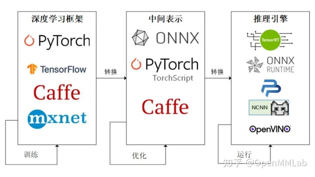
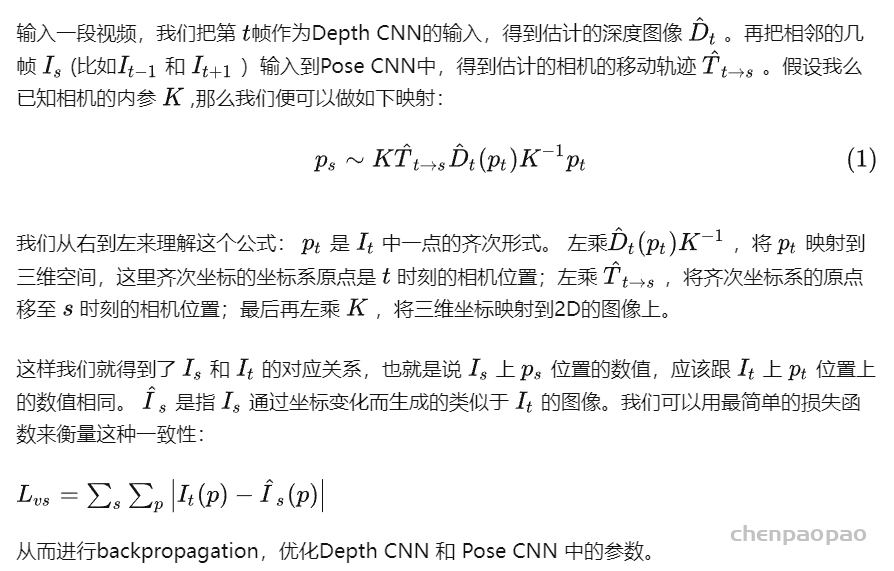
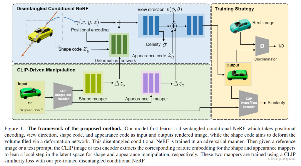
深度学习的工作流程,如下图所示,可分为训练和推理两个部分。
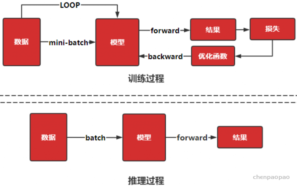
训练过程通过设定数据处理方式,并设计合适的网络模型结构以及损失函数和优化算法,在此基础上将数据集以小批量的方式(mini-batch)反复进行前向计算并计算损失,然后 反向计算梯度利用特定的优化函数来更新模型,来使得损失函数达到最优的结果。训练过程最重要的就是梯度的计算和反向传播。
而推理就是在训练好的模型结构和参数基础上,做一次前向传播得到模型输出的过程。相对于训练而言,推理不涉及梯度和损失优化。推理的最终目标是将训练好的模型部署生产环境中。
高性能推理引擎的工作项
虽然推理就是数据经过模型的一次前向计算,但是推理是面向不同的终端部署,一般推理需要满足:
- 精度要求: 推理的精度需要和训练的精度保持一致,
- 效率要求:性能尽可能的快
- 异构的推理设备:生产环境因为场景不同,支持不同的设备如TPU,CPU,GPU, NPU等
所以推理框架一般包括模型优化和推理加速,以便于支持高性能的推理要求。
那么一个推理框架要做哪些事情呢?
首先,因为推理框架要支持现有流行的深度学习框架如TensorFlow和Pytorch等,而不同的深度学习框内在的不一致性,就要求推理框架需要有一种同一个表达形式,来统一外部的不一致性,这就需要推理框架外部模型解析和转换为内在形式的功能。
其次,为了追求性能的提升,需要能够对训练好的模型针对特定推理设备进行特定的优化,主要优化可以包括
- 低精度优化:FP16低精度转换,INT8后训练量化
- 算子编译优化
- 内存优化
- 计算图调度
低精度优化
一般模型训练过程中都是采用FP32或者FP64高精度的方式进行存储模型参数,主要是因为梯度计算更新的可能是很小的一个小数。高精度使得模型更大,并且计算很耗时。而在推理不需要梯度更新,所以通常如果精度从FP32降低到FP16,模型就会变小很多,并且计算量也下降,而相对于模型的推理效果几乎不会有任何的变化,一般都会做FP16的精度裁剪。
而FP32如果转换到INT8,推理性能会提高很多,但是裁剪不是直接裁剪,参数变动很多,会影响模型的推理效果,需要做重新的训练,来尽可能保持模型的效果
算子编译优化
我们先来了解下计算图的概念,计算图是由算子和张量构建成一个数据计算流向图,通常深度学习网络都可以看成一个计算图。而推理可以理解成数据从计算图起点到终点的过程。
算子编译优化其中一项优化就是计算图的优化。计算图优化的目标是对计算图进行等价的组合变换,使得减少算子的读写操作提供效率。
最简单的情况,就是算子融合。比如常见Conv+ReLu的两个算子,因为Conv需要做大量卷积计算,需要密集的计算单元支持,而Relu几乎不需要计算,如果Relu算子单独运算,则不仅需要一个计算单元支持其实不需要怎么计算的算子,同时又要对前端的数据进行一次读操作,很浪费资源和增加I/O操作; 此时,可以将Conv和Relu合并融合成一个算子,可以节省I/O访问和带宽开销,也可以节省计算单元。
这种算子融合对于所有推理设备都是支持,是通用的硬件优化。有些是针对特定硬件优化,比如某些硬件的计算单元不支持过大算子输入,此时就需要对算子进行拆解。
计算图的优化可以总结为算子拆解、算子聚合、算子重建,以便达到在硬件设备上更好的性能。
算子编译优化的另一个优化就是数据排布优化。我们知道,在TensorFlow框架的输入格式NHWC,而pytorch是NCHW。这些格式是框架抽象出来的矩阵格式,实际在内存中的存储都是按照1维的形式存储。这就涉及物理存储和逻辑存储之间的映射关系,如何更好的布局数据能带来存储数据的访问是一个优化方向;另外在硬件层面,有些硬件在某种存储下有最佳的性能,通常可以根据硬件的读写特点进行优化。
内存优化
我们推理的时候都需要借助额外的硬件设备来达到高速推理,如GPU,NPU等,此时就需要再CPU和这些硬件设备进行交互;以GPU为例,推理时需要将CPU中的数据copy到GPU显存中,然后进行模型推理,推理完成后的数据是在GPU显存中,此时又需要将GPU显存中的数据copy回cpu中。
这个过程就涉及到存储设备的申请、释放以及内存对齐等操作,而这部分也是比较耗时的。
因此内存优化的方向,通常是减少频繁的设备内存空间的申请和尽量做到内存的复用。
一般的,可以根据张量生命周期来申请空间:
- 静态内存分配:比如一些固定的算子在整个计算图中都会使用,此时需要再模型初始化时一次性申请完内存空间,在实际推理时不需要频繁申请操作,提高性能
- 动态内存分配:对于中间临时的内存需求,可以进行临时申请和释放,节省内存使用,提高模型并发能力
- 内存复用:对于同一类同一个大小的内存形式,又满足临时性,可以复用内存地址,减少内存申请。
计算图调度
在计算图中,存在某些算子是串行依赖,而某些算子是不依赖性;这些相互独立的子计算图,就可以进行并行计算,提高推理速度,这就是计算图的调度。
TensorRT
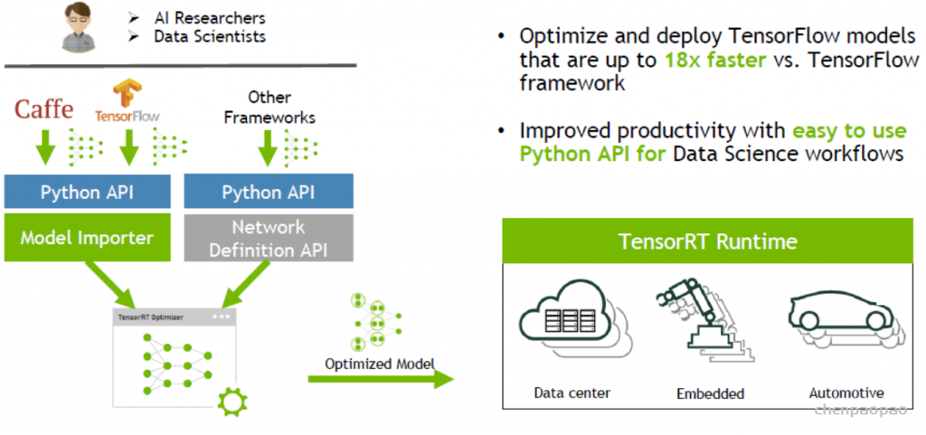
我们讲解了推理引擎的一般工作流程和优化思路,这一部分介绍一个具体的推理引擎框架:TensorRT。NVIDIA TensorRT 是一个用于深度学习推理的 SDK 。 TensorRT 提供了 API 和解析器,可以从所有主要的深度学习框架中导入经过训练的模型。然后,它生成可在数据中心以及汽车和嵌入式环境中部署的优化运行时引擎。TensorRT是NVIDIA出品的针对深度学习的高性能推理SDK。
目前,TensorRT只支持NVIDIA自家的设备的推理服务,如服务器GPUTesla v100、NVIDIA GeForce系列以及支持边缘的NVIDIA Jetson等。
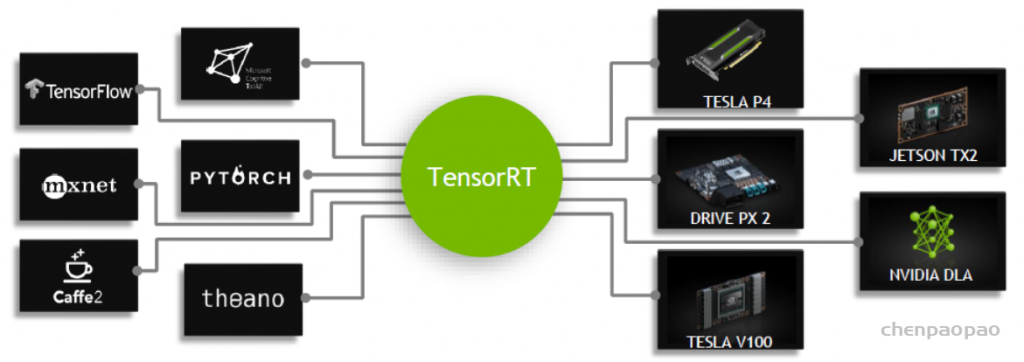
TensorRT通过将现有深度学习框架如TensorFlow、mxnet、pytorch、caffe2以及theano等训练好的模型进行转换和优化,并生成TensorRT的运行时(Runtime Engine),利用TensorRT提供的推理接口(支持不同前端语言如c++/python等),部署不同的NVIDIA GPU设备上,提供高性能人工智能的服务。
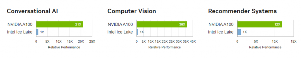
在性能方面,TensorRT在自家的设备上提供了优越的性能:
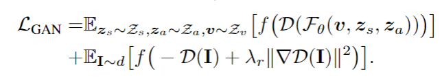
对于TensorRT而言,主要优化如下:
- 算子和张量的融合 Layer & Tensor Fusion
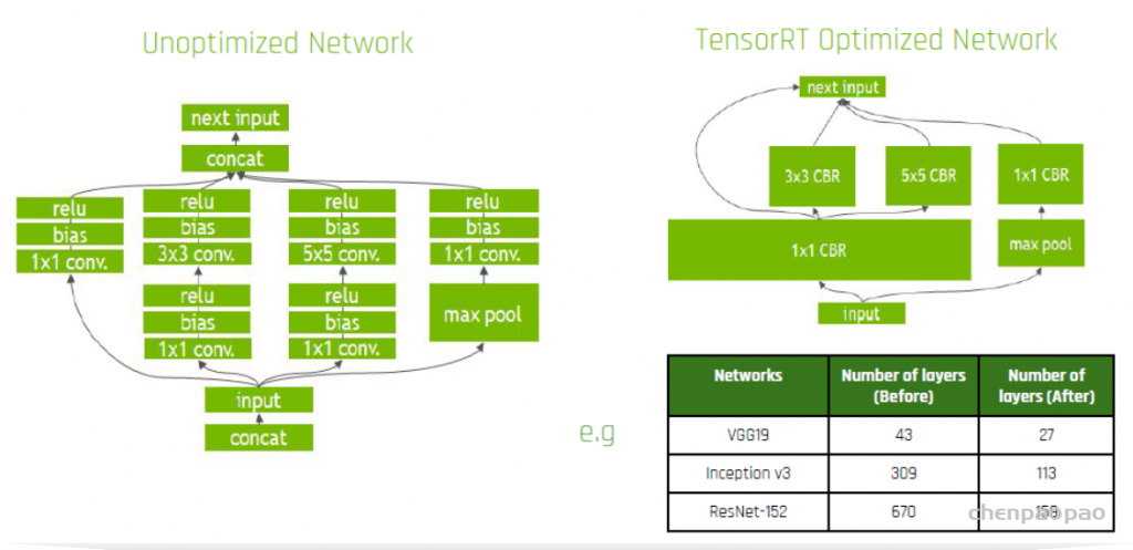
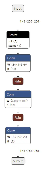
以上面Inception模块的计算图为例子,左边是未优化原始的结构图,右边是经过TensorRT优化过的计算图。优化的目标是减少GPU核数的使用,以便于减少GPU核计算需要的数据读写,提高GPU核数的计算效率
- 首先是合并conv+bias+relu为一个CBR模块,减少2/3 核的使用
- 然后是对于同一输入1x1conv,合并为一个大的CBR,输出保持不变,减少了2次的相同数据的读写
- 有没有发现还少了一个concat层,这个是怎么做到的?concat操作可以理解为数据的合并,TensorRT采用预先先申请足够的缓存,直接把需要concat的数据放到相应的位置就可以达到concat的效果。
经过优化,使得整个模型层数更少,占用更少GPU核,运行效率更快。
- 精度裁剪 Precision Calibration
这个是所有推理引擎都有部分,TensorRT支持低精度FP16和INT8的模型精度裁剪,在尽量不降低模型性能的情况,通过裁剪精度,降低模型大小,提供推理速度。但需要注意的是:不一定FP16就一定比FP32的要快。这取决于设备的不同精度计算单元的数量,比如在GeForce 1080Ti设备上由于FP16的计算单元要远少于FP32的,裁剪后反而效率降低,而GeForce 2080Ti则相反。 - Dynamic Tensor Memory: 这属于提高内存利用率
- Multi-Stream Execution: 这属于内部执行进程控制,支持多路并行执行,提供效率
- Auto-Tuning 可理解为TensorRT针对NVIDIA GPU核,设计有针对性的GPU核优化模型,如上面所说的算子编译优化。
TensorRT安装
了解了TensorRT是什么和如何做优化,我们实际操作下TensorRT, 先来看看TensorRT的安装。
TensorRT是针对NVIDIA GPU的推理引擎,所以需要CUDA和cudnn的支持,需要注意版本的对应关系; 以TensorRT 7.1.3.4为例,需要至少CUDA10.2和cudnn 8.x。
本质上 TensorRT的安装包就是动态库文件(CUDA和cudnn也是如此),需要注意的是TensorRT提供的模型转换工具。
下载可参考
rpm -i cuda-repo-rhel7-10-2-local-10.2.89-440.33.01-1.0-1.x86_64.rpm
tar -zxvf cudnn-10.2-linux-x64-v8.0.1.13.tgz
# tar -xzvf TensorRT-${version}.Linux.${arch}-gnu.${cuda}.${cudnn}.tar.gz
tar -xzvf TensorRT-7.1.3.4.CentOS-7.6.x86_64-gnu.cuda-10.2.cudnn8.0.tar.gz
TensorRT也提供了python版本(底层还是c的动态库)
#1.创建虚拟环境 tensorrt
  conda create -n tensorrt python=3.6

  #安装其他需要的工具包, 按需包括深度学习框架
  pip install keras,opencv-python,numpy,tensorflow-gpu==1.14,pytorch,torchvision

#2. 安装pycuda
  #首先使用nvcc确认cuda版本是否满足要求: nvcc -V
  pip install 'pycuda>=2019.1.1'

#3. 安装TensorRT
  # 下载解压的tar包
  tar -xzvf TensorRT-7.1.3.4.CentOS-7.6.x86_64-gnu.cuda-10.2.cudnn8.0.tar.gz

  #解压得到 TensorRT-7.1.3.4的文件夹,将里面lib绝对路径添加到环境变量中
  export LD_LIBRARY_PATH=$LD_LIBRARY_PATH:/usr/local/TensorRT-7.1.3.4/lib

  #安装TensorRT
  cd TensorRT-7.1.3.4/python
  pip install pip install tensorrt-7.1.3.4-cp36-none-linux_x86_64.whl

#4.安装UFF
  cd TensorRT-7.1.3.4/uff
  pip install uff-0.6.9-py2.py3-none-any.whl

#5. 安装graphsurgeon
  cd TensorRT-7.1.3.4/graphsurgeon
  pip install uff-0.6.9-py2.py3-none-any.whl

#6. 环境测试
  #进入python shell,导入相关包没有报错,则安装成功
  import tensorrt
  import uff
安装完成后,在该路径的samples/python给了很多使用tensorrt的python接口进行推理的例子(图像分类、目标检测等),以及如何使用不同的模型解析接口(uff,onnx,caffe)。
另外给了一个common.py文件,封装了tensorrt如何为engine分配显存,如何进行推理等操作,我们可以直接调用该文件内的相关函数进行tensorrt的推理工作。
TensorRT工作流程
在安装TensorRT之后,如何使用TensorRT呢?我们先来了解下TensorRT的工作流程
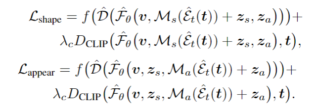
总体流程可以拆分成两块:
- 模型转换
TensorRT需要将不同训练框架训练出来的模型,转换为TensorRT支持的中间表达(IR),并做计算图的优化等,并序列化生成plan文件。

- 模型推理:在模型转换好后之后,在推理时,需要加plan文件进行反序列化加载模型,并通过TensorRT运行时进行模型推理,输出结果

模型转换
由于不同的深度学习框架的实现逻辑不同,TensorRT在转换模型时采用不同适配方法。以当前最流行深度学习框架TensorFlow和Pytorch为例为例。
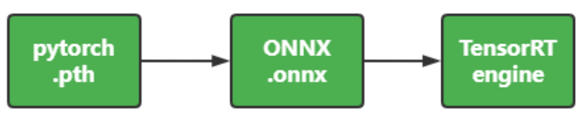
由于pytorch采用动态的计算图,也就是没有图的概念,需要借助ONNX生成静态图。
Open Neural Network Exchange(ONNX,开放神经网络交换)格式,是一个用于表示深度学习模型的标准,可使模型在不同框架之间进行转移.最初的ONNX专注于推理(评估)所需的功能。 ONNX解释计算图的可移植,它使用graph的序列化格式
pth 转换为onnx
import onnx
import torch
def export_onnx(onnx_model_path, model, cuda, height, width, dummy_input=None):
    model.eval()
    if dummy_input is None:
        dummy_input = torch.randn(1, 3, height, width).float()
    dummy_input.requires_grad = True
    print("dummy_input shape: ", dummy_input.shape, dummy_input.requires_grad)

    if cuda:
        dummy_input = dummy_input.cuda()

    torch.onnx.export(
        model,  # model being run
        dummy_input,  # model input (or a tuple for multiple inputs)
        onnx_model_path,  # where to save the model (can be a file or file-like object)
        export_params=True,  # store the trained parameter weights inside the model file
        opset_version=10,  # the ONNX version to export the model to
        do_constant_folding=True,  # whether to execute constant folding for optimization
        verbose=True,
        input_names=['input'],  # the model's input names
        output_names=['output'],  # the model's output names
    )
从上可知,onnx通过pytorch模型完成一次模型输入和输出的过程来遍历整个网络的方式来构建完成的计算图的中间表示。
这里需要注意三个重要的参数:
- opset_version: 这个是onnx支持的op算子的集合的版本,因为onnx目标是在不同深度学习框架之间做模型转换的中间格式,理论上onnx应该支持其他框架的所有算子,但是实际上onnx支持的算子总是滞后的,所以需要知道那个版本支持什么算子,如果转换存在问题,大部分当前的版本不支持需要转换的算子。
- input_names:模型的输入,如果是多个输入,用列表的方式表示,如[“input”, “scale”]
- output_names: 模型的输出, 多个输出,通input_names
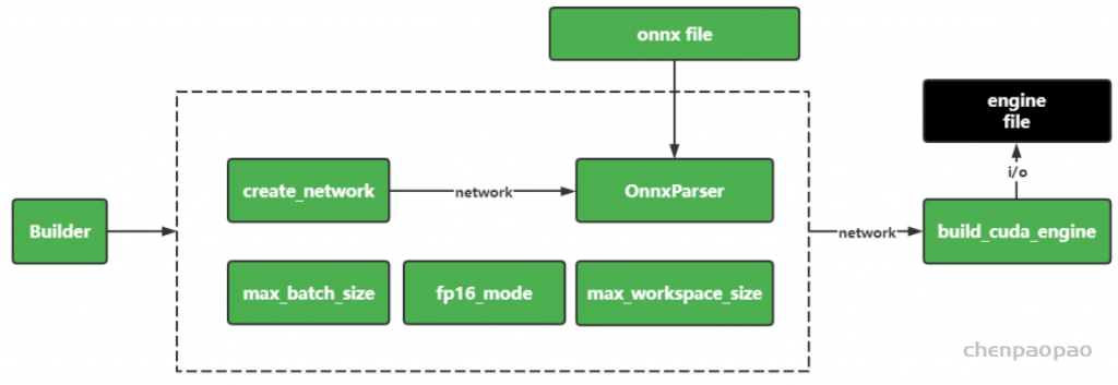
onnx转换为plan engine模型
这里给出的通过TensorRT的python接口来完成onnx到plan engine模型的转换。
import tensorrt as trt
def build_engine(onnx_path):
          EXPLICIT_BATCH = 1 << (int)(trt.NetworkDefinitionCreationFlag.EXPLICIT_BATCH)
        with trt.Builder(TRT_LOGGER) as builder, builder.create_network(EXPLICIT_BATCH) as network, trt.OnnxParser(network, TRT_LOGGER) as parser:
            builder.max_batch_size = 128
            builder.max_workspace_size = 1<<15
            builder.fp16_mode = True
            builder.strict_type_constraints = True
            with open(onnx_path, 'rb') as model:
                parser.parse(model.read())
            # Build and return an engine.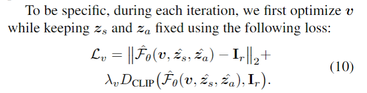
return builder.build_cuda_engine(network)从上面的转换过程可知,TensortRT的转换涉及到几个关键的概念:builder 、 network 、parser
- builder:TensorRT构建器,在构建器中设置模型,解析器和推理的参数设置等
trt.Builder(TRT_LOGGER) - network: TensorRT能识别的模型结构(计算图)
- parser:这里是指解析onnx模型结构(计算图)
从总体上看,TensorRT的转换模型是,将onnx的模型结构(以及参数)转换到TensorRT的network中,同时设置模型推理和优化的参数(如精度裁剪等)。 用一张图来总结下上述过程:
保存engine和读取engine
#解析模型,构建engine并保存
with build_engine(onnx_path) as engine:
    with open(engine_path, "wb") as f:
        f.write(engine.serialize())

#直接加载engine
with open(engine_path, "rb") as f, trt.Runtime(TRT_LOGGER) as runtime:
    engine = runtime.deserialize_cuda_engine(f.read())
TensorFlow / Keras

TensorFlow或者Keras(后台为TensorFlow)采用的是静态的计算图,本身就有图的完整结构,一般模型训练过程会保留ckpt格式,有很多冗余的信息,需要转换为pb格式。针对TensorFlow,TensorRT提供了两种转换方式,一种是pb直接转换,这种方式加速效果有限所以不推荐;另一种是转换uff格式,加速效果明显。
- 转换为pb
from tensorflow.python.framework import graph_io
from tensorflow.python.framework import graph_util
from tensorflow.python.platform import gfile
# 设置输出节点为固定名称
OUTPUT_NODE_PREFIX = 'output_'
NUMBER_OF_OUTPUTS = 1
#输入和输出节点名称
output_names = ['output_']
input_names = ['input_']
input_tensor_name = input_names[0] + ":0"
output_tensor_name = output_names[0] + ":0"

def keras_to_pb(model_path, pb_path):
    K.clear_session()#可以保持输入输出节点的名称每次执行都一致
    K.set_learning_phase(0)
    sess = K.get_session()
    try:
        model = load_model(model_path)# h5 model file_path
    except ValueError as err:
        print('Please check the input saved model file')
        raise err

    output = [None]*NUMBER_OF_OUTPUTS
    output_node_names = [None]*NUMBER_OF_OUTPUTS
    for i in range(NUMBER_OF_OUTPUTS):
        output_node_names[i] = OUTPUT_NODE_PREFIX+str(i)
        output[i] = tf.identity(model.outputs[i], name=output_node_names[i])

    try:
        frozen_graph = graph_util.convert_variables_to_constants(sess, sess.graph.as_graph_def(), output_node_names)
        graph_io.write_graph(frozen_graph, os.path.dirname(pb_path), os.path.basename(pb_path), as_text=False)
        print('Frozen graph ready for inference/serving at {}'.format(pb_path))
    except:
print("error !")- pb 到uff
采用TensorRT提供的uff模块的from_tensorflow_frozen_model()将pb格式模型转换成uff格式模型
import uff
def pb_to_uff(pb_path, uff_path, output_names):
        uff_model = uff.from_tensorflow_frozen_model(pb_path, output_names, output_filename=uff_path)
uff转换成plan engine模型
import tensorrt as trt

TRT_LOGGER = trt.Logger(trt.Logger.INFO)
img_size_tr = (3,224,224) #CHW
input_names = ['input_0']
output_names = ['output_0']

def build_engine(uff_path):
    with trt.Builder(TRT_LOGGER) as builder, builder.create_network() as network, trt.UffParser() as parser:
        builder.max_batch_size = 128 #must bigger than batch_size
        builder.max_workspace_size =1<<15  #cuda buffer size
        builder.fp16_mode = True  #set dtype: fp32, fp16, int8
        builder.strict_type_constraints = True
        # Parse the Uff Network
        parser.register_input(input_names[0], img_size_tr)#NCHW
        parser.register_output(output_names[0])
        parser.parse(uff_path, network)
        # Build and return an engine.
        return builder.build_cuda_engine(network)
在绑定完输入输出节点之后,parser.parse()可以解析uff格式文件,并保存相应网络到network。而后通过builder.build_cuda_engine()得到可以直接在cuda执行的engine文件。该engine文件的构建需要一定时间,可以保存下来,下次直接加载该文件,而不需要解析模型后再构建。
TensorFlow的模型转换基本和onnx是一样的,主要是解析器不一样是UffParser。
#解析模型,构建engine并保存
with build_engine(uff_path) as engine:
    with open(engine_path, "wb") as f:
        f.write(engine.serialize())

#直接加载engine
with open(engine_path, "rb") as f, trt.Runtime(TRT_LOGGER) as runtime:
    engine = runtime.deserialize_cuda_engine(f.read())
模型推理
通过TensorRT的模型转换后,外部训练好的模型都被TensorRT统一成TensorRT可识别的engine文件(并优化过)。在推理时,只要通过TensorRT的推理SDK就可以完成推理。
具体的推理过程如下:
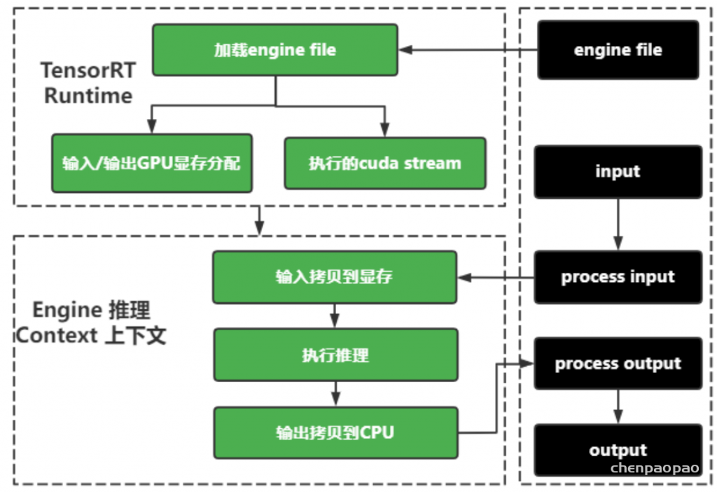
- 通过TensorRT运行时,加载转换好的engine
- 推理前准备:(1)在CPU中处理好输入(如读取数据和标准化等)(2)利用TensorRT的推理SDK中common模块进行输入和输出GPU显存分配
- 执行推理:(1)将CPU的输入拷贝到GPU中 (2)在GPU中进行推理,并将模型输出放入GPU显存中
- 推理后处理:(1)将输出从GPU显存中拷贝到CPU中 (2)在CPU中进行其他后处理
import common
import numpy as np
import cv2
import tensorrt as trt

def inference_test(engine_path, img_file):

    # process input
    input_image = cv2.imread(img_file)
    input_image = input_image[..., ::-1] / 255.0
    input_image = np.expand_dims(input_image, axis=0)

    input_image = input_image.transpose((0, 3, 1, 2))  # NCHW for pytorch
    input_image = input_image.reshape(1, -1)  # .ravel()

    # infer
    batch_size = 1
    TRT_LOGGER = trt.Logger(trt.Logger.INFO)
    with open(engine_path, "rb") as f, trt.Runtime(TRT_LOGGER) as runtime:
        engine = runtime.deserialize_cuda_engine(f.read())
        # Allocate buffers and create a CUDA stream
        inputs, outputs, bindings, stream = common.allocate_buffers(engine, batch_size)
        # Contexts are used to perform inference.
        with engine.create_execution_context() as context:
             np.copyto(inputs[0].host, input_image)
             [output] = common.do_inference(context, bindings=bindings, inputs=inputs, outputs=outputs, stream=stream, batch_size=batch_size)
TensorRT进阶和缺点
前面较全面了介绍了TensorRT的特点(优点)和工作流程;希望能感受到TensorRT的魅力所在。
在实际代码中主要是通过python的接口来讲解,TensorRT也提供了C++的转换和推理方式,但是主要的关键概念是一样
那TensorRT有什么局限性吗?
首先,TensorRT只支持NVIDIA自家的设备,并根据自家设备的特点,做了很多的优化,如果是其他设备,TensorRT就不适用了。这时候可以考虑其他的推理框架,比如以推理编译为基础的TVM, 针对移动平台推理NCNN,MACE、MNN以及TFLite等,以及针对Intel CPU的OPENVINO。
其次,算子的支持程度;这几乎是所有第三方推理框架都遇到的问题,TensorRT在某些不支持的算子的情况下,TensorRT提供了plugin的方式,plugin提供了标准接口,允许自己开发新的算子,并以插件的方式加入TensorRT(后面会专门介绍,欢迎关注)。
总结
- 训练需要前向计算和反向梯度更新,推理只需要前向计算
- 推理框架优化:低精度优化、算子编译优化、内存优化、计算图调度
- TensorRT是针对NVIDIA设备的高性能推理框架
- TensorRT工作流程包括模型转换和模型推理
- 针对Pytorch, TensorRT模型转换链路为:pth->onnx->trt plan
- 针对TensorFlow,TensorRT模型转换链路为:ckpt->pb->uff->trt plan
- TensorRT模型转换关键点为build,network和parse
- TensorRT模型推理关键点为:tensorrt runtime,engine context,显存操作和推理