SfM(Structure from motion) 是一种三维重建的方法,用于从motion中实现3D重建。也就是从时间系列的2D图像中推算3D信息。
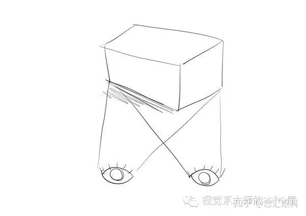
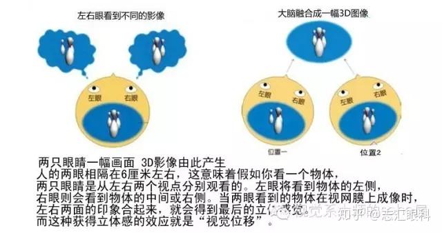
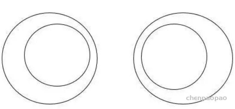
人的大脑可以从动的物体中取得其三维的信息,是因为大脑在动的2D图像中找到了匹配的地方,即Corresponding area (points)。然后通过匹配点之间的视差得到相对的深度信息,在这一点上,原理和基于Stereo的三维重建相同。
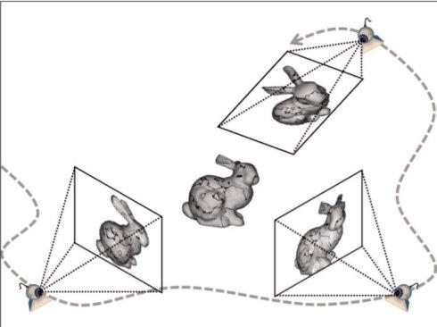
SfM的输入是一段motion或者一时间系列的2D图群,如下图所示 [1],这里不需要任何相机的信息。然后通过2D图之间的匹配可以推断出相机的各项参数。Corresponding points可以用SIFT,SURF来匹配,也可以用最新的AKAZE(SIFT的改进版,2010)来匹配。而Corresponding points的跟踪则可以用Lucas-Kanede的Optical Flow来完成。
在SfM中,误匹配会造成较大的Error,所以要对匹配进行筛选,目前流行的方法是RANSAC(Random Sample Consensus)。2D的误匹配点可以应用3D的Geometric特征来进行排除。
Bundler [2] 就是一种SfM的方法,Bundler使用了基于SIFT的匹配算法,并且对匹配进行了过滤去噪处理。下图显示了一组测试数据(一时间系列的2D图群):
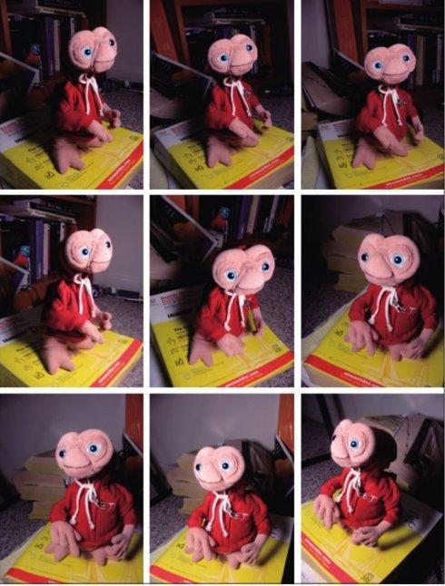
将这些图片保存到同一个文件夹,然后将文件夹的目录输入,Bundler会自行处理,之后会得到一群Corresponding points。比如其中的一组Corresponding points (A1,A2,A3,…Am),其实他们来自同一个三维点A的Projection。所以通过这些点可以重建三维点A。然后将很多组Corresponding points 进行重建,则得到了一群三维的点,这里称为3D点阵。
然后3D点阵可以通过MeshLab(开源Source,支持Windows/Linux/Mac)来重建稀疏的Mesh。也可以通过PMVS(Patch-based Multi-view Stereo)来重建Dense的Mesh[3]。
[1] 満上育久 ”Structure from Motion – Osaka University“ 映像情报メディア学会志 Vol.65, No.4, pp.479-482, 2011.
[2] N.Snavely, S.M. Seitz, R.Szeliski, “Modeling the World from Internet Photo Collections”, International Journal of Computer Vision, vol.80, no.2, 2008.
[3] Y. Furukawa, J.Ponce, “Accurate, Dense and Robust Multi-view Stereopsis” IEEE Transactions on Pattern Analysis and Machine Intelligence, 2009.
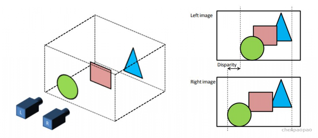
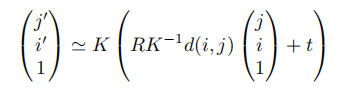
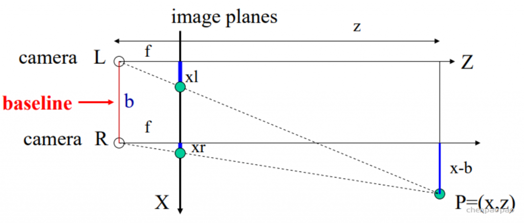
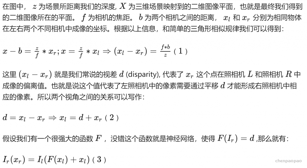
补充:通过视差d求解深度图:
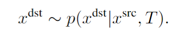
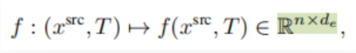
同一水平线上的两个照相机拍摄到的照片是服从以下物理规律的:
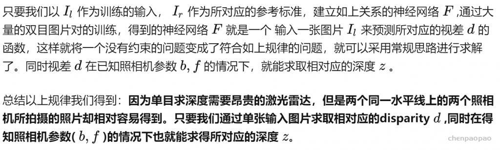
这种思路最先应用于使用单张图片生成新视角问题:DeepStereo 和 Deep3d之中, 在传统的视角生成问题之中,首先会利用两张图(或多张)求取图片之间的视差d,其次通过得到的视差(相当于三维场景)来生成新视角