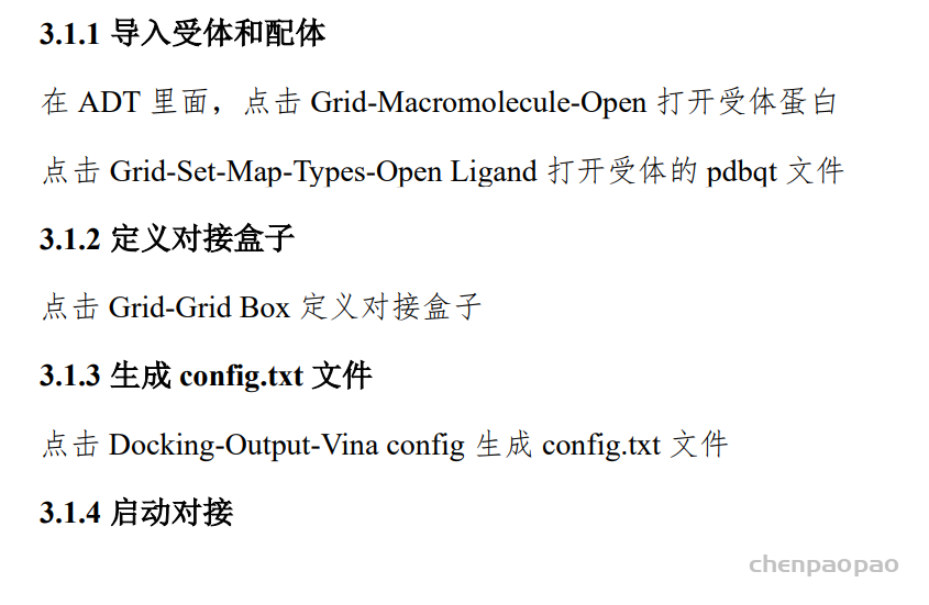
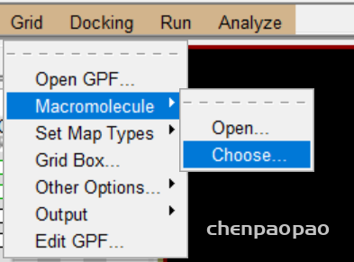
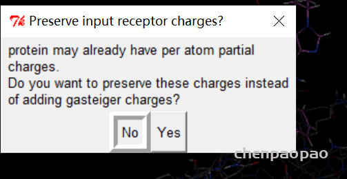
import gym

from stable_baselines import DQN
from stable_baselines.common.evaluation import evaluate_policy


# Create environment
env = gym.make('LunarLander-v2')

# Instantiate the agent
model = DQN('MlpPolicy', env, learning_rate=1e-3, prioritized_replay=True, verbose=1)
# Train the agent
model.learn(total_timesteps=int(2e5))
# Save the agent
model.save("dqn_lunar")
del model  # delete trained model to demonstrate loading

# Load the trained agent
model = DQN.load("dqn_lunar")

# Evaluate the agent
mean_reward, std_reward = evaluate_policy(model, model.get_env(), n_eval_episodes=10)

# Enjoy trained agent
obs = env.reset()
for i in range(1000):
    action, _states = model.predict(obs)
    obs, rewards, dones, info = env.step(action)
    env.render()
fromstable_baselines.common.cmd_utilimport make_atari_env
fromstable_baselines.common.vec_envimport VecFrameStack
fromstable_baselinesimport ACER
# There already exists an environment generator# that will make and wrap atari environments correctly.# Here we are also multiprocessing training (num_env=4 => 4 processes)
env = make_atari_env('PongNoFrameskip-v4', num_env=4, seed=0)
# Frame-stacking with 4 frames
env = VecFrameStack(env, n_stack=4)
model = ACER('CnnPolicy', env, verbose=1)
model.learn(total_timesteps=25000)
obs = env.reset()
whileTrue:
action, _states = model.predict(obs)
obs, rewards, dones, info = env.step(action)
env.render()
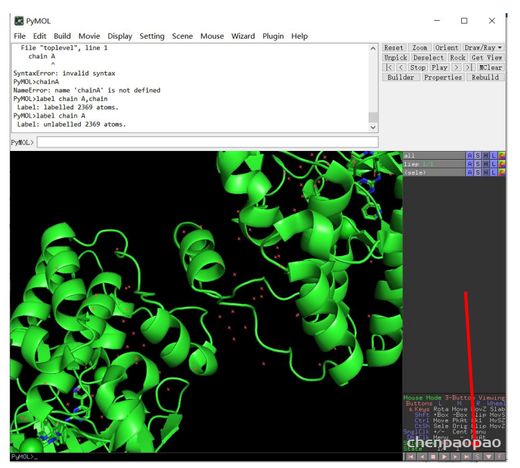
bug解决:
在执行时:
import gym
env = gym.make('ALE/Pong-v5')
env.reset()

for i in range(1000):
    env.step(env.action_space.sample())
    env.render()
env.close()
输出,无法对fream进行渲染。
ImportError: cannot import name ‘rendering’ from ‘gym.envs.classic_control’.
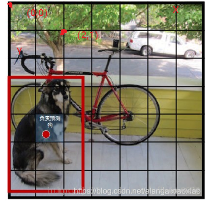
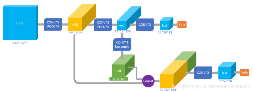
每个 bounding box 要预测 (x, y, w, h) 和 confidence 共5个值,每个网格还要预测一个类别信息,记为 C 类。则 SxS个 网格,每个网格要预测 B 个 bounding box, 每个box中都有 C 个 classes对应的概率值。输出就是 S x S x B x(5+C) 的一个 tensor。
void forward_convolutional_layer(convolutional_layer l, network_state state)
{
int out_h = convolutional_out_height(l);//获得本层卷积层输出特征图的高、宽
int out_w = convolutional_out_width(l);
int i, j;
// l.outputs = l.out_h * l.out_w * l.out_c在make各网络层函数中赋值(比如make_convolutional_layer()),// 对应每张输入图片的所有输出特征图的总元素个数(每张输入图片会得到n也即l.out_c张特征图)// 初始化输出l.output全为0.0;输入l.outputs*l.batch为输出的总元素个数,其中l.outputs为batch// 中一个输入对应的输出的所有元素的个数,l.batch为一个batch输入包含的图片张数;0表示初始化所有输出为0;
fill_cpu(l.outputs*l.batch, 0, l.output, 1);//将地址l.output,l.outputs*l.batch个float地址空间的数据初始化0
.......
作者在进行卷积运算前,将输入特征图进行重新排序:
```c
void im2col_cpu(float* data_im,
int channels, int height, int width,
int ksize, int stride, int pad, float* data_col)
{
int c,h,w;
// 计算该层神经网络的输出图像尺寸(其实没有必要再次计算的,因为在构建卷积层时,make_convolutional_layer()函数// 已经调用convolutional_out_width(),convolutional_out_height()函数求取了这两个参数,// 此处直接使用l.out_h,l.out_w即可,函数参数只要传入该层网络指针就可了,没必要弄这么多参数)
int height_col = (height + 2*pad - ksize) / stride + 1;
int width_col = (width + 2*pad - ksize) / stride + 1;
/// 卷积核大小:ksize*ksize是一个卷积核的大小,之所以乘以通道数channels,是因为输入图像有多通道,每个卷积核在做卷积时,/// 是同时对同一位置处多通道的图像进行卷积运算,这里为了实现这一目的,将三通道上的卷积核并在一起以便进行计算,因此卷积核/// 实际上并不是二维的,而是三维的,比如对于3通道图像,卷积核尺寸为3*3,该卷积核将同时作用于三通道图像上,这样并起来就得/// 到含有27个元素的卷积核,且这27个元素都是独立的需要训练的参数。所以在计算训练参数个数时,一定要注意每一个卷积核的实际/// 训练参数需要乘以输入通道数。
int channels_col = channels * ksize * ksize;//输入通道// 外循环次数为一个卷积核的尺寸数,循环次数即为最终得到的data_col的总行数
for (c = 0; c < channels_col; ++c) {
//行,列偏置都是对应着本次循环要操作的输出位置的像素而言的,通道偏置,是该位置像素所在的输出通道的绝对位置(通道数)// 列偏移,卷积核是一个二维矩阵,并按行存储在一维数组中,利用求余运算获取对应在卷积核中的列数,比如对于// 3*3的卷积核(3通道),当c=0时,显然在第一列,当c=5时,显然在第2列,当c=9时,在第二通道上的卷积核的第一列,// 当c=26时,在第三列(第三输入通道上)
int w_offset = c % ksize;//0,1,2// 行偏移,卷积核是一个二维的矩阵,且是按行(卷积核所有行并成一行)存储在一维数组中的,// 比如对于3*3的卷积核,处理3通道的图像,那么一个卷积核具有27个元素,每9个元素对应一个通道上的卷积核(互为一样),// 每当c为3的倍数,就意味着卷积核换了一行,h_offset取值为0,1,2,对应3*3卷积核中的第1, 2, 3行
int h_offset = (c / ksize) % ksize;//0,1,2// 通道偏移,channels_col是多通道的卷积核并在一起的,比如对于3通道,3*3卷积核,每过9个元素就要换一通道数,// 当c=0~8时,c_im=0;c=9~17时,c_im=1;c=18~26时,c_im=2,操作对象是排序后的像素位置
int c_im = c / ksize / ksize;
// 中循环次数等于该层输出图像行数height_col,说明data_col中的每一行存储了一张特征图,这张特征图又是按行存储在data_col中的某行中
for (h = 0; h < height_col; ++h) {
// 内循环等于该层输出图像列数width_col,说明最终得到的data_col总有channels_col行,height_col*width_col列
for (w = 0; w < width_col; ++w) {
// 由上面可知,对于3*3的卷积核,行偏置h_offset取值为0,1,2,当h_offset=0时,会提取出所有与卷积核第一行元素进行运算的像素,// 依次类推;加上h*stride是对卷积核进行行移位操作,比如卷积核从图像(0,0)位置开始做卷积,那么最先开始涉及(0,0)~(3,3)// 之间的像素值,若stride=2,那么卷积核进行一次行移位时,下一行的卷积操作是从元素(2,0)(2为图像行号,0为列号)开始
int im_row = h_offset + h * stride;//yolov3-tiny stride = 1// 对于3*3的卷积核,w_offset取值也为0,1,2,当w_offset取1时,会提取出所有与卷积核中第2列元素进行运算的像素,// 实际在做卷积操作时,卷积核对图像逐行扫描做卷积,加上w*stride就是为了做列移位,// 比如前一次卷积其实像素元素为(0,0),若stride=2,那么下次卷积元素起始像素位置为(0,2)(0为行号,2为列号)
int im_col = w_offset + w * stride;
// col_index为重排后图像中的像素索引,等于c * height_col * width_col + h * width_col +w(还是按行存储,所有通道再并成一行),// 对应第c通道,h行,w列的元素
int col_index = (c * height_col + h) * width_col + w;//将重排后的图片像素,按照左上->右下的顺序,计算一维索引//im_col + width*im_row + width*height*channel 重排前的特征图在内存中的位置索引// im2col_get_pixel函数获取输入图像data_im中第c_im通道,im_row,im_col的像素值并赋值给重排后的图像,// height和width为输入图像data_im的真实高、宽,pad为四周补0的长度(注意im_row,im_col是补0之后的行列号,// 不是真实输入图像中的行列号,因此需要减去pad获取真实的行列号)
data_col[col_index] = im2col_get_pixel(data_im, height, width, channels,
im_row, im_col, c_im, pad);
// return data_im[im_col + width*im_row + width*height*channel)];
}
}
}
}
通过gemm进行卷积乘加操作,通过add_bias添加偏置。
//进行卷积的乘加运算,没有bias偏置参数参与运算;
gemm(0, 0, m, n, k, 1, a, k, b, n, 1, c, n);

add_bias(l.output, l.biases, l.batch, l.n, out_h*out_w);//每个输出特征图的元素都加上对应通道的偏置参数
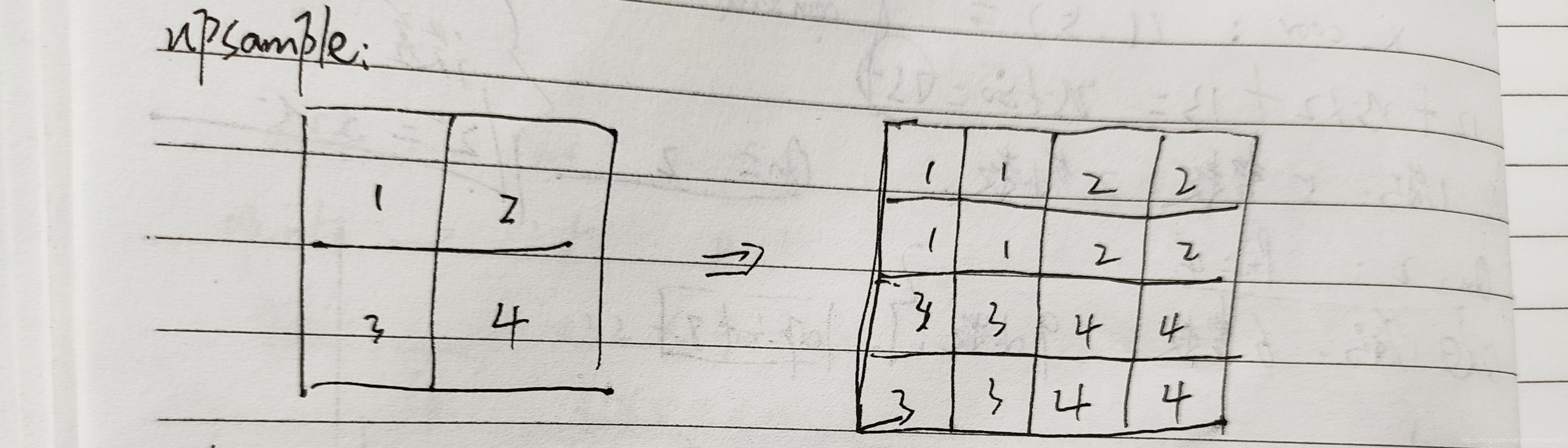
void upsample_cpu(float *in, int w, int h, int c, int batch, int stride, int forward, float scale, float *out)
{

    int i, j, k, b;
    for (b = 0; b < batch; ++b) {
        for (k = 0; k < c; ++k) {
            for (j = 0; j < h*stride; ++j) {
                for (i = 0; i < w*stride; ++i) {
                    int in_index = b*w*h*c + k*w*h + (j / stride)*w + i / stride;
                    int out_index = b*w*h*c*stride*stride + k*w*h*stride*stride + j*w*stride + i;
                    if (forward) out[out_index] = scale*in[in_index];
                    else in[in_index] += scale*out[out_index];
                }
            }
        }
    }
}
//w,h:640,424 netw, neth:416,416 thresh:图像置信度阈值0.25 hier:0.5//map:0 relative:1 letter:0//根据yolo层 计算满足置信度阈值要求的box相对的预测坐标、宽度和高度,并将结果保存在dets[count].bbox结构体中//每个box有80个类别,有一个置信度,该类别对应的可能性prob:class概率*置信度///舍弃prob小于阈值0.25的box
int get_yolo_detections(layer l, int w, int h, int netw, int neth, float thresh, int *map, int relative, detection *dets, int letter)
{
printf("\n l.batch = %d, l.w = %d, l.h = %d, l.n = %d ,netw = %d, neth = %d \n", l.batch, l.w, l.h, l.n, netw, neth);
int i,j,n;
float *predictions = l.output;//yolo层的输出// This snippet below is not necessary// Need to comment it in order to batch processing >= 2 images//if (l.batch == 2) avg_flipped_yolo(l);
int count = 0;
//printf("yolo layer l.mask[0] is %d, l.mask[1] is %d, l.mask[2] is %d\n", l.mask[0], l.mask[1], l.mask[2]);//printf("yolo layer l.biases[l.mask[0]*2] is %f, l.biases[l.mask[1]*2] is %f, l.biases[l.mask[2]*2] is %f\n", l.biases[l.mask[0] * 2], l.biases[l.mask[1] * 2], l.biases[l.mask[2] * 2]);//遍历yolo层
for (i = 0; i < l.w*l.h; ++i){//该yolo层输出特征图的宽度、高度:13x13 26x26
int row = i / l.w;
int col = i % l.w;
for(n = 0; n < l.n; ++n){//yolo层,l.n = 3//obj_index:置信度层索引
int obj_index = entry_index(l, 0, n*l.w*l.h + i, 4);//obj_index = n*l.w*l.h*(4+l.classes+1) + 4*l.w*l.h + i;
float objectness = predictions[obj_index];//获得对应的置信度//if(objectness <= thresh) continue; // incorrect behavior for Nan values
if (objectness > thresh) {//只有置信度大于阈值才开始执行该分支//printf("\n objectness = %f, thresh = %f, i = %d, n = %d \n", objectness, thresh, i, n);//box_index:yolo层每个像素点有三个box,表示每个box的索引值
int box_index = entry_index(l, 0, n*l.w*l.h + i, 0);//box_index = n*l.w*l.h*(4+l.classes+1)+ i;//l.biases->偏置参数起始地址 l.mask[n]:分别为3,4,5,0,1,2,biases偏置参数偏移量//根据yolo层 计算满足置信度阈值要求的box相对的预测坐标、宽度和高度,并将结果保存在dets[count].bbox结构体中
dets[count].bbox = get_yolo_box(predictions, l.biases, l.mask[n], box_index, col, row, l.w, l.h, netw, neth, l.w*l.h);
//获取对应的置信度,该置信度经过了logistic
dets[count].objectness = objectness;
//获得分类数:80(int类型)
dets[count].classes = l.classes;
for (j = 0; j < l.classes; ++j) {
//80个类别,每个类别对应的概率,class_index为其所在层的索引
int class_index = entry_index(l, 0, n*l.w*l.h + i, 4 + 1 + j);//class_index = n*l.w*l.h*(4+l.classes+1) + (4+1+j)*l.w*l.h + i;//每个box有80个类别,有一个置信度,该类别对应的可能性prob:class概率*置信度
float prob = objectness*predictions[class_index];
//舍弃prob小于阈值0.25的box
dets[count].prob[j] = (prob > thresh) ? prob : 0;
}
++count;
}
}
}
correct_yolo_boxes(dets, count, w, h, netw, neth, relative, letter);
return count;
}
非极大值抑制[NMS]
//dets:box结构体 nboxes:满足阈值的box个数 l.classe:80 thresh=0.45f//两个box,同一类别进行非极大值抑制,遍历
void do_nms_sort(detection *dets, int total, int classes, float thresh)
{
int i, j, k;
k = total - 1;
for (i = 0; i <= k; ++i) {//box个数
if (dets[i].objectness == 0) {//置信度==0 不执行该分支,理论上没有objectness = 0
printf("there is no objectness == 0 !!! \n");
detection swap = dets[i];
dets[i] = dets[k];
dets[k] = swap;
--k;
--i;
}
}
total = k + 1;
//同一类别进行比较
for (k = 0; k < classes; ++k) {//80个 //box预测的类别
for (i = 0; i < total; ++i) {//box个数
dets[i].sort_class = k;
}
//函数作用:将prob较大的box排列到前面
qsort(dets, total, sizeof(detection), nms_comparator_v3);
for (i = 0; i < total; ++i) {//两个box,同一类别进行非极大值抑制//printf(" k = %d, \t i = %d \n", k, i);
if (dets[i].prob[k] == 0) continue;
box a = dets[i].bbox;
for (j = i + 1; j < total;++j){
box b = dets[j].bbox;
if( box_iou(a, b) > thresh) dets[j].prob[k] = 0;
}
}
}
}
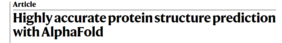
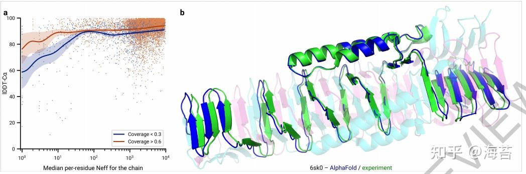
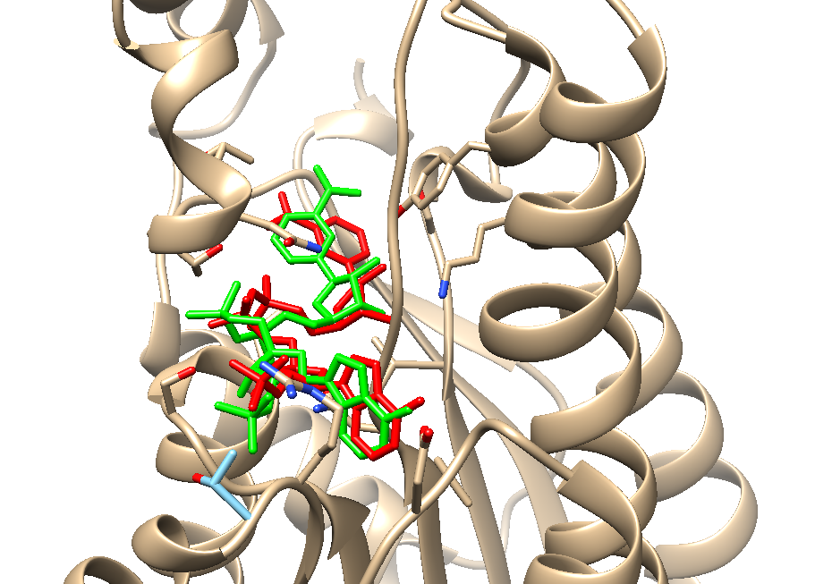
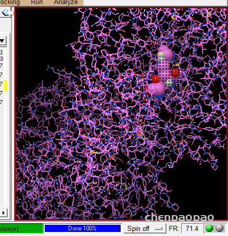
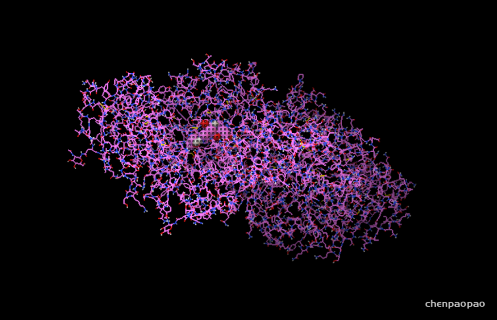
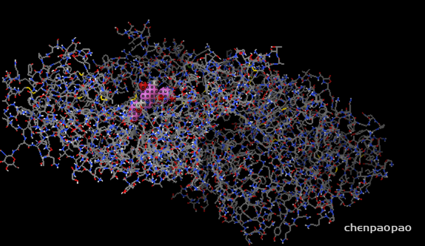
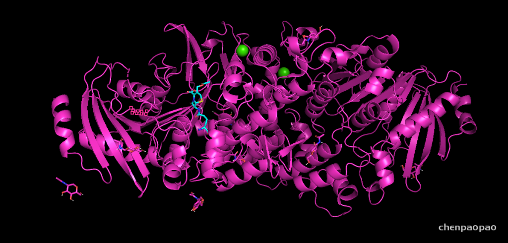
Fig. 1 | AlphaFold produces highly accurate structures.
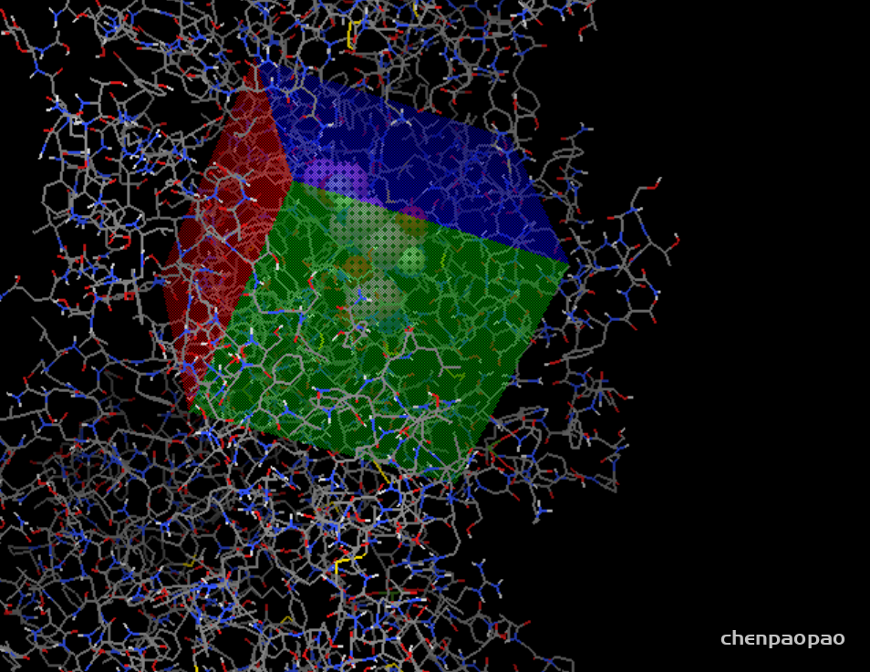
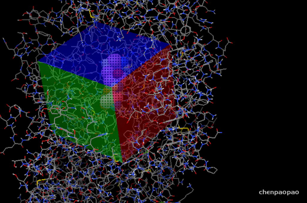
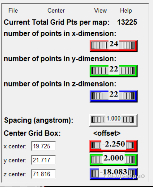
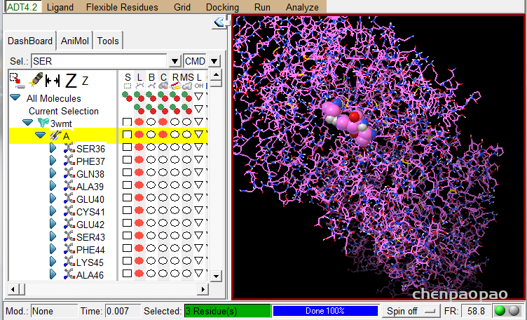
PDB蛋白质结构数据库(Protein Data Bank,简称PDB)是美国Brookhaven国家实验室于1971年创建的,由结构生物信息学研究合作组织(Research Collaboratory for Structural Bioinformatics,简称RCSB)维护。和核酸序列数据库一样,可以通过网络直接向PDB数据库提交数据。
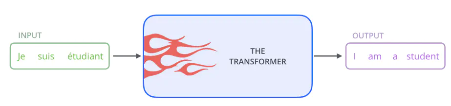
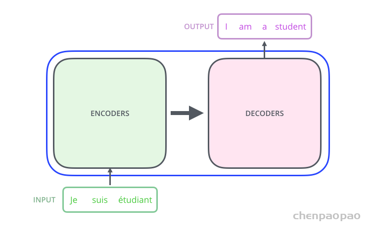
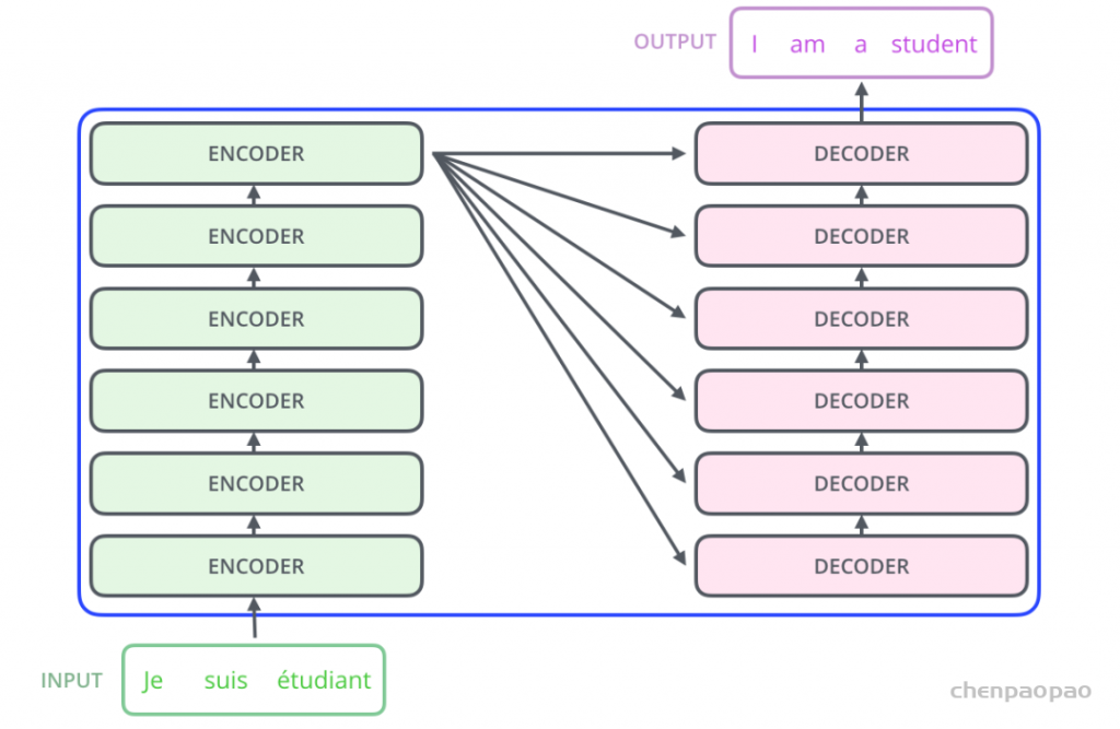
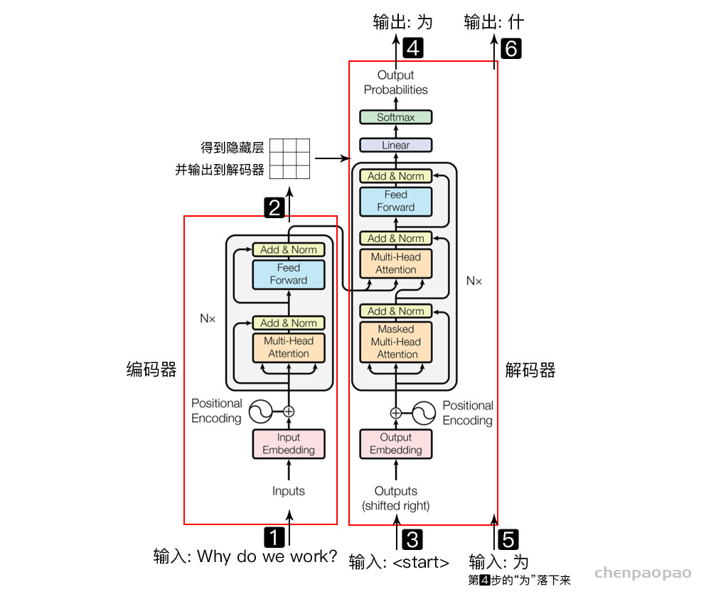
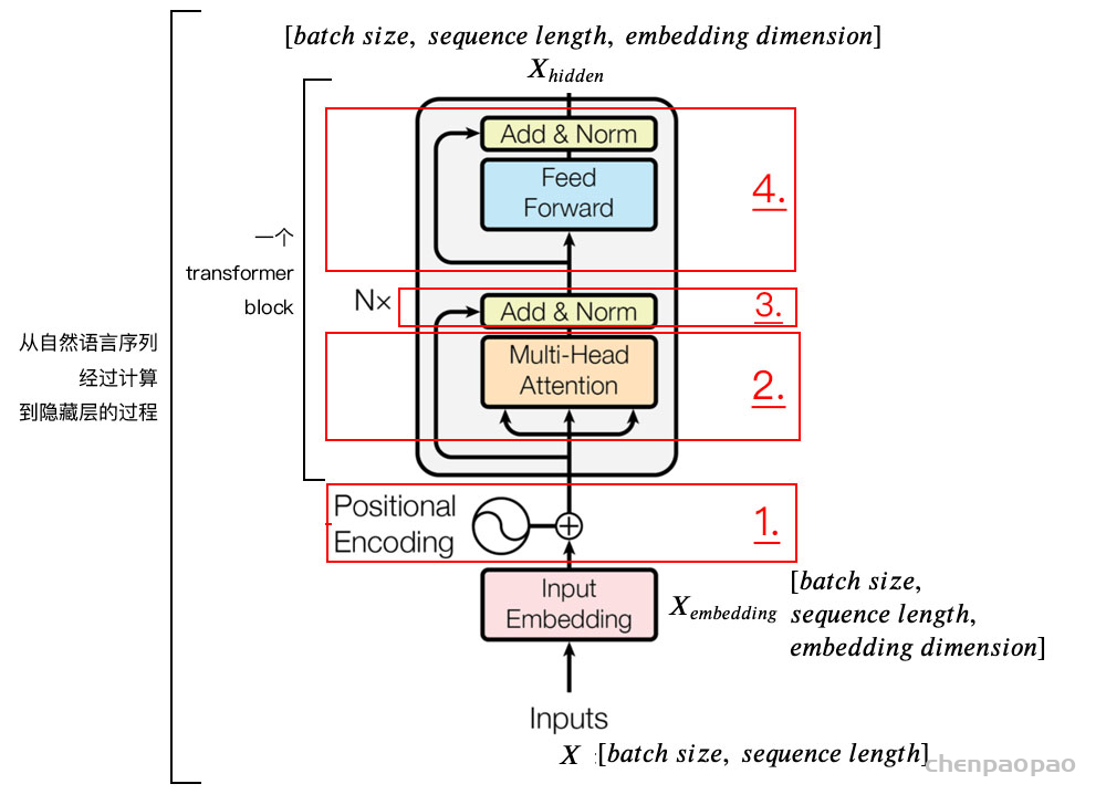
Why do we work?,我们为什么工作?左侧红框是编码器,右侧红框是解码器,编码器负责把自然语言序列映射成为隐藏层(上图第2步),即含有自然语言序列的数学表达。解码器把隐藏层再映射为自然语言序列,从而使我们可以解决各种问题,如情感分析、机器翻译、摘要生成、语义关系抽取等。简单说下,上图每一步都做了什么:
Why do we work?,我们为什么工作?左侧红框是编码器,右侧红框是解码器,编码器负责把自然语言序列映射成为隐藏层(上图第2步),即含有自然语言序列的数学表达。解码器把隐藏层再映射为自然语言序列,从而使我们可以解决各种问题,如情感分析、机器翻译、摘要生成、语义关系抽取等。简单说下,上图每一步都做了什么:
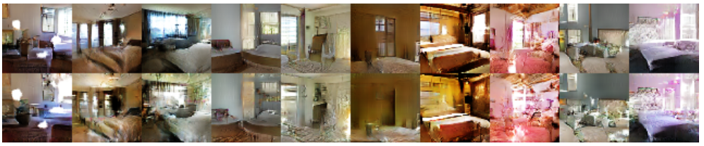
首先,类似于 cGAN ,随机产生一些噪声,然后串联图像A以生成伪图像 B ^ ,之后,使用来自 VAE-GAN 的同一编码器将伪图像 B ^ 编码为潜矢量。 最后,从编码的潜矢量中采样 z ^ ,并用输入噪声 z 计算损失。数据流为 z −> B ^ −> z ^ ( 图(d) 中的实线箭头),有两个损失:
对抗损失 \(L_{GAN}\)
噪声 N(z) 与潜在编码之间的 L1损失 \(L_{1}^{latent}\)
通过组合这两个数据流,在输出和潜在空间之间得到了一个双映射循环。 BicycleGAN 中的 bi 来自双映射(双向单射),这是一个数学术语,简单来说其表示一对一映射,并且是可逆的。在这种情况下,BicycleGAN 将输出映射到潜在空间,并且类似地从潜在空间映射到输出。总损失如下:


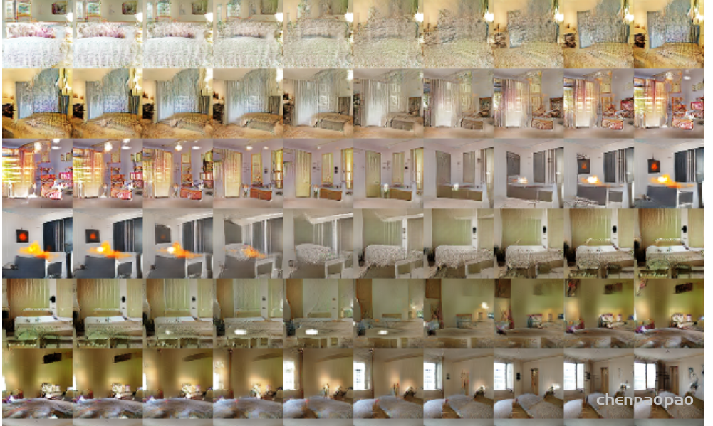


 。 此时为了衡量重构和真实的误差,这里用了L1损失和GAN的对抗思想实现,我们在后面损失函数分析部分再说。这样cVAE-GAN部分就可以训练了,cVAE GAN的重点还是在得到的embedding z。