Paper: https://arxiv.org/abs/2010.02502
Code: https://github.com/ermongroup/ddim
摘自:扩散模型之DDIM
在 DDPM 中,生成过程被定义为马尔可夫扩散过程的反向过程,在逆向采样过程的每一步,模型预测噪声
DDIM 的作者发现,扩散过程并不是必须遵循马尔科夫链, 在之后的基于分数的扩散模型以及基于随机微分等式的理论都有相同的结论。 基于此,DDIM 的作者重新定义了扩散过程和逆过程,并提出了一种新的采样技巧, 可以大幅减少采样的步骤,极大的提高了图像生成的效率,代价是牺牲了一定的多样性, 图像质量略微下降,但在可接受的范围内。
对于扩散模型来说,一个最大的缺点是需要设置较长的扩散步数才能得到好的效果,这导致了生成样本的速度较慢,比如扩散步数为1000的话,那么生成一个样本就要模型推理1000次。这篇文章我们将介绍另外一种扩散模型DDIM(Denoising Diffusion Implicit Models),DDIM和DDPM有相同的训练目标,但是它不再限制扩散过程必须是一个马尔卡夫链,这使得DDIM可以采用更小的采样步数来加速生成过程,DDIM的另外是一个特点是从一个随机噪音生成样本的过程是一个确定的过程(中间没有加入随机噪音)。
前提条件:1.马尔可夫过程。2.微小噪声变化。
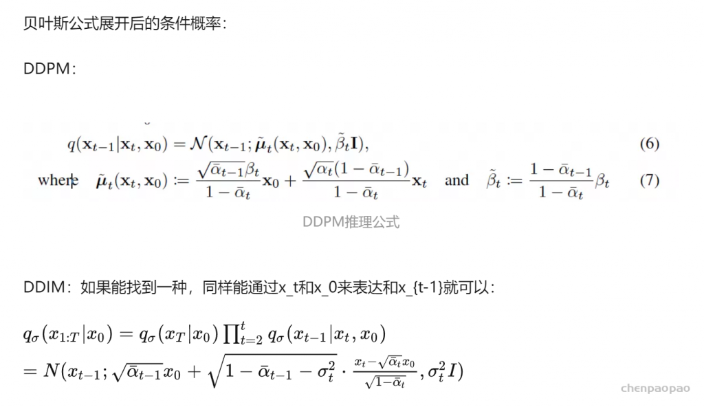
步骤一:在DDPM中我们基于初始图像状态以及最终高斯噪声状态,通过贝叶斯公式以及多元高斯分布的散度公式,可以计算出每一步骤的逆向分布。之后继续重复上述对逆向分布的求解步骤,最终实现从纯高斯噪声,恢复到原始图片的步骤。
步骤二:模型优化部分通过最小化分布的交叉熵,预测出模型逆向分布的均值和方差,将其带入步骤一中的推理过程即可。
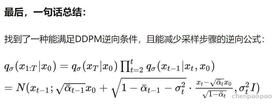
文章中存在的一个核心问题是:由于1.每个步骤都是马尔可夫链。2.每次加特征的均值和方差都需要控制在很小的范围下。因此我们不得不每一步都进行逆向的推理和运算,导致模型整体耗时很长。本文核心针对耗时问题进行优化,一句话总结:在满足DDPM中逆向推理的条件下,找到一种用 xt 和 x0 表达 xt−1 且能能大幅减少计算量的推理方式。

代码实现:
DDIM和DDPM的训练过程一样,所以可以直接在DDPM的基础上加一个新的生成方法(这里主要参考了DDIM官方代码以及diffusers库),具体代码如下所示:
class GaussianDiffusion:
    def __init__(self, timesteps=1000, beta_schedule='linear'):
     pass

    # ...

 # use ddim to sample
    @torch.no_grad()
    def ddim_sample(
        self,
        model,
        image_size,
        batch_size=8,
        channels=3,
        ddim_timesteps=50,
        ddim_discr_method="uniform",
        ddim_eta=0.0,
        clip_denoised=True):
        # make ddim timestep sequence
        if ddim_discr_method == 'uniform':
            c = self.timesteps // ddim_timesteps
            ddim_timestep_seq = np.asarray(list(range(0, self.timesteps, c)))
        elif ddim_discr_method == 'quad':
            ddim_timestep_seq = (
                (np.linspace(0, np.sqrt(self.timesteps * .8), ddim_timesteps)) ** 2
            ).astype(int)
        else:
            raise NotImplementedError(f'There is no ddim discretization method called "{ddim_discr_method}"')
        # add one to get the final alpha values right (the ones from first scale to data during sampling)
        ddim_timestep_seq = ddim_timestep_seq + 1
        # previous sequence
        ddim_timestep_prev_seq = np.append(np.array([0]), ddim_timestep_seq[:-1])

        device = next(model.parameters()).device
        # start from pure noise (for each example in the batch)
        sample_img = torch.randn((batch_size, channels, image_size, image_size), device=device)
        for i in tqdm(reversed(range(0, ddim_timesteps)), desc='sampling loop time step', total=ddim_timesteps):
            t = torch.full((batch_size,), ddim_timestep_seq[i], device=device, dtype=torch.long)
            prev_t = torch.full((batch_size,), ddim_timestep_prev_seq[i], device=device, dtype=torch.long)

            # 1. get current and previous alpha_cumprod
            alpha_cumprod_t = self._extract(self.alphas_cumprod, t, sample_img.shape)
            alpha_cumprod_t_prev = self._extract(self.alphas_cumprod, prev_t, sample_img.shape)

            # 2. predict noise using model
            pred_noise = model(sample_img, t)

            # 3. get the predicted x_0
            pred_x0 = (sample_img - torch.sqrt((1. - alpha_cumprod_t)) * pred_noise) / torch.sqrt(alpha_cumprod_t)
            if clip_denoised:
                pred_x0 = torch.clamp(pred_x0, min=-1., max=1.)

            # 4. compute variance: "sigma_t(η)" -> see formula (16)
            # σ_t = sqrt((1 − α_t−1)/(1 − α_t)) * sqrt(1 − α_t/α_t−1)
            sigmas_t = ddim_eta * torch.sqrt(
                (1 - alpha_cumprod_t_prev) / (1 - alpha_cumprod_t) * (1 - alpha_cumprod_t / alpha_cumprod_t_prev))

            # 5. compute "direction pointing to x_t" of formula (12)
            pred_dir_xt = torch.sqrt(1 - alpha_cumprod_t_prev - sigmas_t**2) * pred_noise

            # 6. compute x_{t-1} of formula (12)
            x_prev = torch.sqrt(alpha_cumprod_t_prev) * pred_x0 + pred_dir_xt + sigmas_t * torch.randn_like(sample_img)

            sample_img = x_prev

        return sample_img.cpu().numpy()
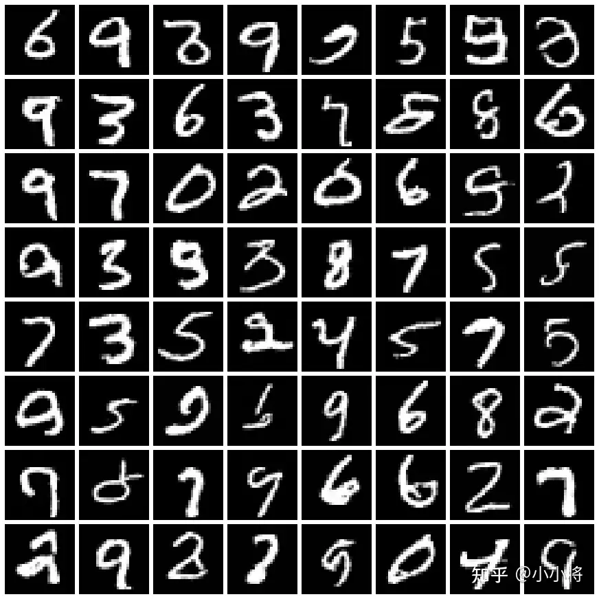
这里以MNIST数据集为例,训练的扩散步数为500,直接采用DDPM(即推理500次)生成的样本如下所示:
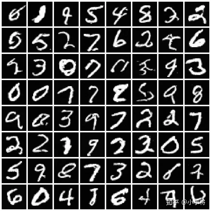
同样的模型,我们采用DDIM来加速生成过程,这里DDIM的采样步数为50,其生成的样本质量和500步的DDPM相当:
完整的代码示例见https://github.com/xiaohu2015/nngen。
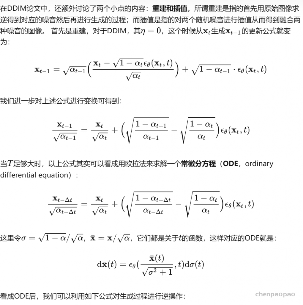
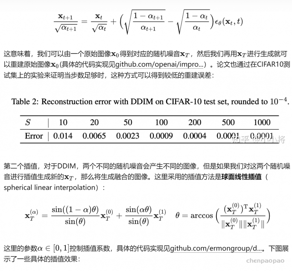
其它:重建和插值
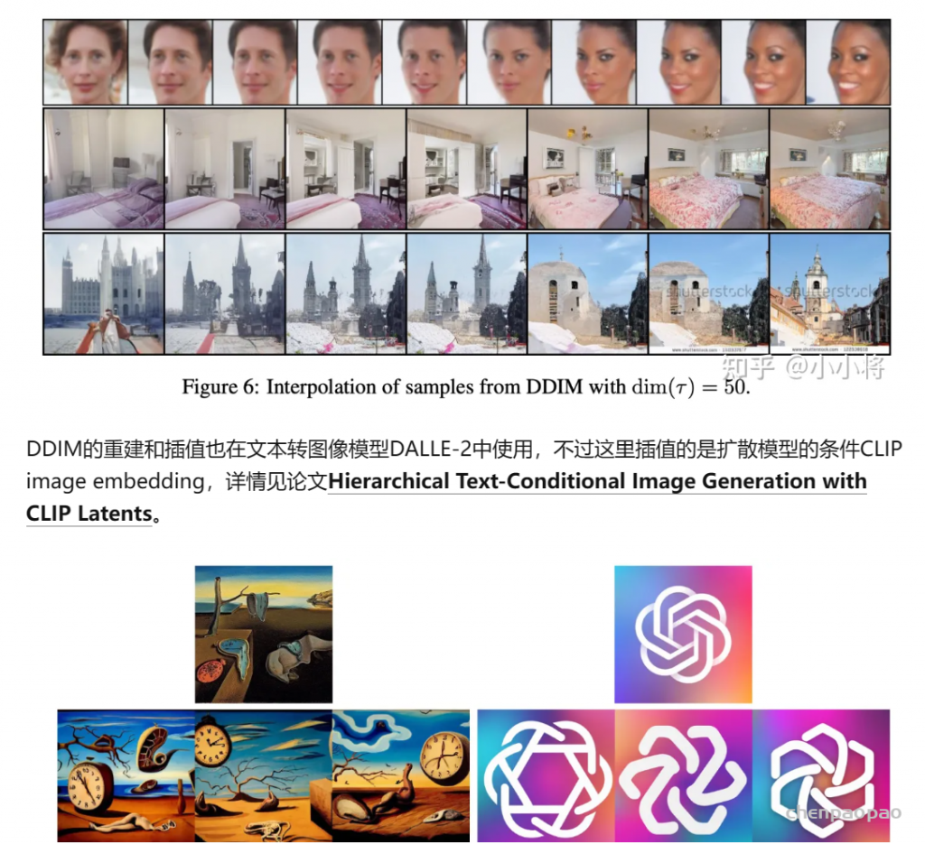
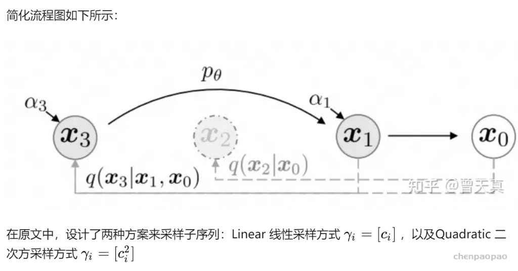
如果从直观上看,DDIM的加速方式非常简单,直接采样一个子序列,其实论文DDPM+也采用了类似的方式来加速。另外DDIM和其它扩散模型的一个较大的区别是其生成过程是确定性的。