PointNet++

论文：https://arxiv.org/abs/1706.02413（NIPS 2017）

code： https://github.com/charlesq34/pointnet2

1、改进

PointNet因为是只使用了MLP和max pooling，没有能力捕获局部结构，因此在细节处理和泛化到复杂场景上能力很有限。

1. point-wise MLP，仅仅是对每个点表征，对局部结构信息整合能力太弱 –> PointNet++的改进：sampling和grouping整合局部邻域
2. global feature直接由max pooling获得，无论是对分类还是对分割任务，都会造成巨大的信息损失 –> PointNet++的改进：hierarchical feature learning framework，通过多个set abstraction逐级降采样，获得不同规模不同层次的local-global feature
3. 分割任务的全局特征global feature是直接复制与local feature拼接，生成discriminative feature能力有限 –> PointNet++的改进：分割任务设计了encoder-decoder结构，先降采样再上采样，使用skip connection将对应层的local-global feature拼接

2、方法

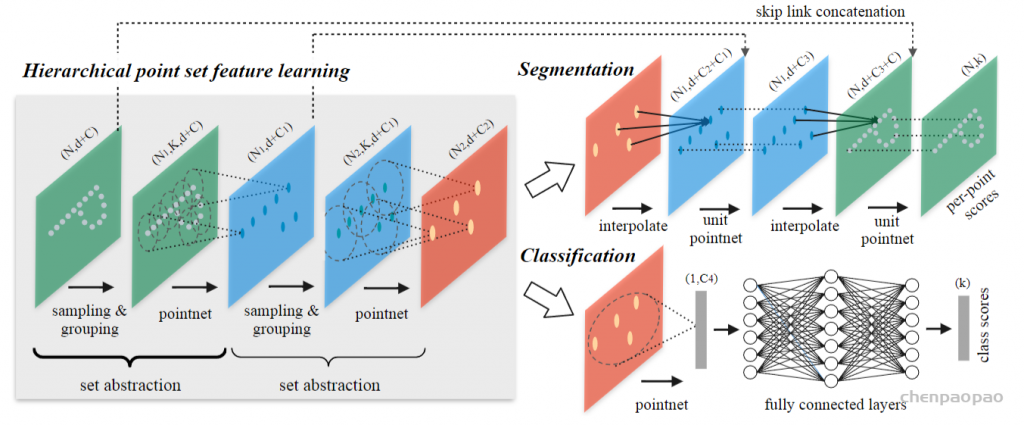
PointNet++的网络大体是encoder-decoder结构

encoder为降采样过程，通过多个set abstraction结构实现多层次的降采样，得到不同规模的point-wise feature，最后一个set abstraction输出可以认为是global feature。其中set abstraction由sampling，grouping，pointnet三个模块构成。

decoder根据分类和分割应用，又有所不同。分类任务decoder比较简单，不介绍了。分割任务decoder为上采样过程，通过反向插值和skip connection实现在上采样的同时，还能够获得local+global的point-wise feature，使得最终的表征能够discriminative（分辩能力）。

思考：

1. PointNet++降采样过程是怎么实现的？/PointNet++是如何表征global feature的？（关注set abstraction, sampling layer, grouping layer, pointnet layer）
2. PointNet++用于分割任务的上采样过程是怎么实现的？/PointNet++是如何表征用于分割任务的point-wise feature的？（关注反向插值，skip connection）

 🐖：上图中的 d 表示坐标空间维度， C 表示特征空间维度

2.1 encoder

在PointNet的基础上增加了hierarchical （层级）feature learning framework的结构。这种多层次的结构由set abstraction层组成。

在每一个层次的set abstraction，点集都会被处理和抽象，而产生一个规模更小的点集，可以理解成是一个降采样表征过程，可参考上图左半部分。

set abstraction由三个部分构成（代码贴在下面）：

def pointnet_sa_module(xyz, points, npoint, radius, nsample, mlp, mlp2, group_all, is_training, bn_decay, scope, bn=True, pooling='max', knn=False, use_xyz=True, use_nchw=False):
    ''' PointNet Set Abstraction (SA) Module
        Input:
            xyz: (batch_size, ndataset, 3) TF tensor
            points: (batch_size, ndataset, channel) TF tensor
            npoint: int32 -- #points sampled in farthest point sampling
            radius: float32 -- search radius in local region
            nsample: int32 -- how many points in each local region
            mlp: list of int32 -- output size for MLP on each point
            mlp2: list of int32 -- output size for MLP on each region
            group_all: bool -- group all points into one PC if set true, OVERRIDE
                npoint, radius and nsample settings
            use_xyz: bool, if True concat XYZ with local point features, otherwise just use point features
            use_nchw: bool, if True, use NCHW data format for conv2d, which is usually faster than NHWC format
        Return:
            new_xyz: (batch_size, npoint, 3) TF tensor
            new_points: (batch_size, npoint, mlp[-1] or mlp2[-1]) TF tensor
            idx: (batch_size, npoint, nsample) int32 -- indices for local regions
    '''
    data_format = 'NCHW' if use_nchw else 'NHWC'
    with tf.variable_scope(scope) as sc:
        # Sample and Grouping
        if group_all:
            nsample = xyz.get_shape()[1].value
            new_xyz, new_points, idx, grouped_xyz = sample_and_group_all(xyz, points, use_xyz)
        else:
            new_xyz, new_points, idx, grouped_xyz = sample_and_group(npoint, radius, nsample, xyz, points, knn, use_xyz)
        # Point Feature Embedding
        if use_nchw: new_points = tf.transpose(new_points, [0,3,1,2])
        for i, num_out_channel in enumerate(mlp):
            new_points = tf_util.conv2d(new_points, num_out_channel, [1,1],
                                        padding='VALID', stride=[1,1],
                                        bn=bn, is_training=is_training,
                                        scope='conv%d'%(i), bn_decay=bn_decay,
                                        data_format=data_format) 
        if use_nchw: new_points = tf.transpose(new_points, [0,2,3,1])
        # Pooling in Local Regions
        if pooling=='max':
            new_points = tf.reduce_max(new_points, axis=[2], keep_dims=True, name='maxpool')
        elif pooling=='avg':
            new_points = tf.reduce_mean(new_points, axis=[2], keep_dims=True, name='avgpool')
        elif pooling=='weighted_avg':
            with tf.variable_scope('weighted_avg'):
                dists = tf.norm(grouped_xyz,axis=-1,ord=2,keep_dims=True)
                exp_dists = tf.exp(-dists * 5)
                weights = exp_dists/tf.reduce_sum(exp_dists,axis=2,keep_dims=True) # (batch_size, npoint, nsample, 1)
                new_points *= weights # (batch_size, npoint, nsample, mlp[-1])
                new_points = tf.reduce_sum(new_points, axis=2, keep_dims=True)
        elif pooling=='max_and_avg':
            max_points = tf.reduce_max(new_points, axis=[2], keep_dims=True, name='maxpool')
            avg_points = tf.reduce_mean(new_points, axis=[2], keep_dims=True, name='avgpool')
            new_points = tf.concat([avg_points, max_points], axis=-1)
        # [Optional] Further Processing 
        if mlp2 is not None:
            if use_nchw: new_points = tf.transpose(new_points, [0,3,1,2])
            for i, num_out_channel in enumerate(mlp2):
                new_points = tf_util.conv2d(new_points, num_out_channel, [1,1],
                                            padding='VALID', stride=[1,1],
                                            bn=bn, is_training=is_training,
                                            scope='conv_post_%d'%(i), bn_decay=bn_decay,
                                            data_format=data_format) 
            if use_nchw: new_points = tf.transpose(new_points, [0,2,3,1])
        new_points = tf.squeeze(new_points, [2]) # (batch_size, npoints, mlp2[-1])
        return new_xyz, new_points, idx

2.1.1 sampling layer

使用FPS（最远点采样）对点集进行降采样，将输入点集从规模 N1 降到更小的规模 N2 。FPS可以理解成是使得采样的各个点之间尽可能远，这种采样的好处是可以降采样结果会比较均匀。

FPS实现方式如下：随机选择一个点作为初始点作为已选择采样点，计算未选择采样点集中每个点与已选择采样点集之间的距离distance，将距离最大的那个点加入已选择采样点集，然后更新distance，一直循环迭代下去，直至获得了目标数量的采样点。

class FarthestSampler:
    def __init__(self):
        pass
    def _calc_distances(self, p0, points):
        return ((p0 - points) ** 2).sum(axis=1)
    def __call__(self, pts, k):
        farthest_pts = np.zeros((k, 3), dtype=np.float32)
        farthest_pts[0] = pts[np.random.randint(len(pts))]
        distances = self._calc_distances(farthest_pts[0], pts)
        for i in range(1, k):
            farthest_pts[i] = pts[np.argmax(distances)]
            distances = np.minimum(
                distances, self._calc_distances(farthest_pts[i], pts))
        return farthest_pts

输入规模为 B∗N∗(d+C) ，其中 B 表示batch size， N 表示点集中点的数量， d 表示点的坐标维度， C 表示点的其他特征（比如法向量等）维度。一般 d=3 ， c=0

输出规模为 B∗N1∗(d+C) ， N1<N ，因为这是一个降采样过程。

sampling和grouping具体实现是写在一个函数里的：

def sample_and_group(npoint, radius, nsample, xyz, points, knn=False, use_xyz=True):
    '''
    Input:
        npoint: int32
        radius: float32
        nsample: int32
        xyz: (batch_size, ndataset, 3) TF tensor
        points: (batch_size, ndataset, channel) TF tensor, if None will just use xyz as points
        knn: bool, if True use kNN instead of radius search
        use_xyz: bool, if True concat XYZ with local point features, otherwise just use point features
    Output:
        new_xyz: (batch_size, npoint, 3) TF tensor
        new_points: (batch_size, npoint, nsample, 3+channel) TF tensor
        idx: (batch_size, npoint, nsample) TF tensor, indices of local points as in ndataset points
        grouped_xyz: (batch_size, npoint, nsample, 3) TF tensor, normalized point XYZs
            (subtracted by seed point XYZ) in local regions
    '''
    new_xyz = gather_point(xyz, farthest_point_sample(npoint, xyz)) # (batch_size, npoint, 3)
    if knn:
        _,idx = knn_point(nsample, xyz, new_xyz)
    else:
        idx, pts_cnt = query_ball_point(radius, nsample, xyz, new_xyz)
    grouped_xyz = group_point(xyz, idx) # (batch_size, npoint, nsample, 3)
    grouped_xyz -= tf.tile(tf.expand_dims(new_xyz, 2), [1,1,nsample,1]) # translation normalization
    if points is not None:
        grouped_points = group_point(points, idx) # (batch_size, npoint, nsample, channel)
        if use_xyz:
            new_points = tf.concat([grouped_xyz, grouped_points], axis=-1) # (batch_size, npoint, nample, 3+channel)
        else:
            new_points = grouped_points
    else:
        new_points = grouped_xyz
    return new_xyz, new_points, idx, grouped_xyz

其中sampling对应的部分是：

new_xyz = gather_point(xyz, farthest_point_sample(npoint, xyz)) # (batch_size, npoint, 3)

xyz既是 B∗N∗3 的点云，npoint是降采样点的规模。注意：PointNet++的FPS均是在坐标空间做的，而不是在特征空间做的。这一点很关键，因为FPS本身是不可微的，无法计算梯度反向传播。

本着刨根问题的心态，我们来看看farthest_point_sample和gather_point究竟在做什么

farthest_point_sample输入输出非常明晰，输出的是降采样点在inp中的索引，因此是 B∗N1 int32类型的张量

def farthest_point_sample(npoint,inp):
    '''
input:
    int32
    batch_size * ndataset * 3   float32
returns:
    batch_size * npoint         int32
    '''
    return sampling_module.farthest_point_sample(inp, npoint)

gather_point的作用就是将上面输出的索引，转化成真正的点云

def gather_point(inp,idx):
    '''
input:
    batch_size * ndataset * 3   float32
    batch_size * npoints        int32
returns:
    batch_size * npoints * 3    float32
    '''
    return sampling_module.gather_point(inp,idx)

2.1.2 grouping layer

上一步sampling的过程是将 N∗(d+C) 降到 N1∗(d+C) （这里论述方便先不考虑batch，就考虑单个点云），实际上可以理解成是在 N 个点中选取 N1 个中心点(key point)。

那么这一步grouping的目的就是以这每个key point为中心，找其固定规模（令规模为 K）的邻点，共同组成一个局部邻域(patch)。也就是会生成 N1 个局部邻域，输出规模为 N1∗K∗(d+C)

if knn:
    _,idx = knn_point(nsample, xyz, new_xyz)
else:
    idx, pts_cnt = query_ball_point(radius, nsample, xyz, new_xyz)
    grouped_xyz = group_point(xyz, idx) # (batch_size, npoint, nsample, 3)

1)找邻域的过程也是在坐标空间进行（也就是以上代码输入输出维度都是 d ，没有 C ， C 是在后面的代码拼接上的），而不是特征空间。

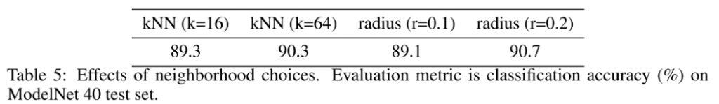
2)找邻域这里有两种方式：KNN和query ball point.

其中前者KNN就是大家耳熟能详的K近邻，找K个坐标空间最近的点。
后者query ball point就是划定某一半径，找在该半径球内的点作为邻点。

还有个问题：query ball point如何保证对于每个局部邻域，采样点的数量都是一样的呢？
事实上，如果query ball的点数量大于规模 K ，那么直接取前 K 个作为局部邻域；如果小于，那么直接对某个点重采样，凑够规模 K

KNN和query ball的区别：（摘自原文）Compared with kNN, ball query’s local neighborhood guarantees a fixed region scale thus making local region feature more generalizable across space, which is preferred for tasks requiring local pattern recognition (e.g. semantic point labeling).也就是query ball更加适合于应用在局部/细节识别的应用上，比如局部分割。

补充材料中也有实验来对比KNN和query ball:

sample_and_group代码的剩余部分：

sample和group操作都是在坐标空间进行的，因此如果还有特征空间信息（即point-wise feature），可以在这里将其与坐标空间拼接，组成新的point-wise feature，准备送入后面的unit point进行特征学习。

if points is not None:
    grouped_points = group_point(points, idx) # (batch_size, npoint, nsample, channel)
    if use_xyz:
        new_points = tf.concat([grouped_xyz, grouped_points], axis=-1) # (batch_size, npoint, nample, 3+channel)
    else:
        new_points = grouped_points
else:
    new_points = grouped_xyz

2.1.3 PointNet layer

使用PointNet对以上结果表征

输入 B∗N∗K∗(d+C) ，输出 B∗N∗(d+C1)

以下代码主要分成3个部分：

1)point feature embedding

这里输入是 B∗N∗K∗(d+C) ，可以类比成是batch size为 B ，宽高为 N∗K ，通道数为 d+C 的图像，这样一类比，这里的卷积就好理解多了实际上就是 1∗1 卷积，不改变feature map大小，只改变通道数，将通道数升高，实现所谓“embedding”

这部分输出是 B∗N∗K∗C1

2)pooling in local regions

pooling，只是是对每个局部邻域pooling,输出是 B∗N∗1∗C1

3)further processing

再对池化后的结果做MLP，也是简单的 1∗1 卷积。这一部分在实际实验中PointNet++并没有设置去做

# Point Feature Embedding
if use_nchw: new_points = tf.transpose(new_points, [0,3,1,2])
for i, num_out_channel in enumerate(mlp):
    new_points = tf_util.conv2d(new_points, num_out_channel, [1,1],
                                padding='VALID', stride=[1,1],
                                bn=bn, is_training=is_training,
                                scope='conv%d'%(i), bn_decay=bn_decay,
                                data_format=data_format) 
if use_nchw: new_points = tf.transpose(new_points, [0,2,3,1])

# Pooling in Local Regions
if pooling=='max':
    new_points = tf.reduce_max(new_points, axis=[2], keep_dims=True, name='maxpool')
elif pooling=='avg':
    new_points = tf.reduce_mean(new_points, axis=[2], keep_dims=True, name='avgpool')
elif pooling=='weighted_avg':
    with tf.variable_scope('weighted_avg'):
        dists = tf.norm(grouped_xyz,axis=-1,ord=2,keep_dims=True)
        exp_dists = tf.exp(-dists * 5)
        weights = exp_dists/tf.reduce_sum(exp_dists,axis=2,keep_dims=True) # (batch_size, npoint, nsample, 1)
        new_points *= weights # (batch_size, npoint, nsample, mlp[-1])
        new_points = tf.reduce_sum(new_points, axis=2, keep_dims=True)
elif pooling=='max_and_avg':
    max_points = tf.reduce_max(new_points, axis=[2], keep_dims=True, name='maxpool')
    avg_points = tf.reduce_mean(new_points, axis=[2], keep_dims=True, name='avgpool')
    new_points = tf.concat([avg_points, max_points], axis=-1)

# [Optional] Further Processing 
if mlp2 is not None:
    if use_nchw: new_points = tf.transpose(new_points, [0,3,1,2])
    for i, num_out_channel in enumerate(mlp2):
        new_points = tf_util.conv2d(new_points, num_out_channel, [1,1],
                                    padding='VALID', stride=[1,1],
                                    bn=bn, is_training=is_training,
                                    scope='conv_post_%d'%(i), bn_decay=bn_decay,
                                    data_format=data_format) 
    if use_nchw: new_points = tf.transpose(new_points, [0,2,3,1])

2.1.4 Encoder还有一个问题

pointnet++实际上就是对局部邻域表征。

那就不得不面对一个挑战：non-uniform sampling density(点云的密度不均匀)，也就是在稀疏点云局部邻域训练可能不能很好挖掘点云的局部结构

PointNet++做法：learn to combine features from regions of different scales when the input sampling density changes.

因此文章提出了两个方案：

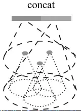
一、Multi-scale grouping（MSG）

对当前层的每个中心点，取不同radius的query ball，可以得到多个不同大小的同心球，也就是得到了多个相同中心但规模不同的局部邻域，分别对这些局部邻域表征，并将所有表征拼接。如上图所示。

该方法比较麻烦，运算较多。

代码层面其实就是加了个遍历radius_list的循环，分别处理，并最后concat

new_xyz = gather_point(xyz, farthest_point_sample(npoint, xyz))
new_points_list = []
for i in range(len(radius_list)):
    radius = radius_list[i]
    nsample = nsample_list[i]
    idx, pts_cnt = query_ball_point(radius, nsample, xyz, new_xyz)
    grouped_xyz = group_point(xyz, idx)
    grouped_xyz -= tf.tile(tf.expand_dims(new_xyz, 2), [1,1,nsample,1])
    if points is not None:
        grouped_points = group_point(points, idx)
        if use_xyz:
            grouped_points = tf.concat([grouped_points, grouped_xyz], axis=-1)
    else:
        grouped_points = grouped_xyz
    if use_nchw: grouped_points = tf.transpose(grouped_points, [0,3,1,2])
    for j,num_out_channel in enumerate(mlp_list[i]):
        grouped_points = tf_util.conv2d(grouped_points, num_out_channel, [1,1],
                                        padding='VALID', stride=[1,1], bn=bn, is_training=is_training,
                                        scope='conv%d_%d'%(i,j), bn_decay=bn_decay)
    if use_nchw: grouped_points = tf.transpose(grouped_points, [0,2,3,1])
    new_points = tf.reduce_max(grouped_points, axis=[2])
    new_points_list.append(new_points)
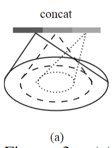
new_points_concat = tf.concat(new_points_list, axis=-1)

二、Multi-resolution grouping（MRG）

（摘自原文）features of a region at some level Li is a concatenation of two vectors.

One vector (left in figure) is obtained by summarizing the features at each subregion from the lower level Li−1 using the set abstraction level.

The other vector (right) is the feature that is obtained by directly processing all raw points in the local region using a single PointNet.

简单来说，就是当前set abstraction的局部邻域表征由两部分构成：

左边表征：对上一层set abstraction（还记得上一层的点规模是更大的吗？）各个局部邻域（或者说中心点）的特征进行聚合。 右边表征：使用一个单一的PointNet直接在局部邻域处理原始点云

2.2 decoder：

2.2.1 分类任务的decoder

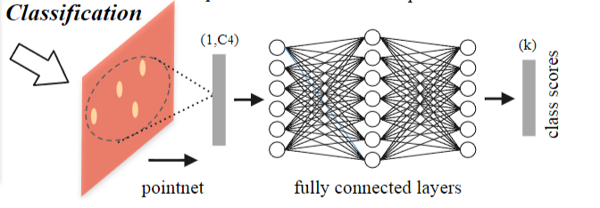
比较简单，将encoder降采样得到的global feature送入几层全连接网络，最后通过一个softmax分类。

2.2.2 分割任务的decoder

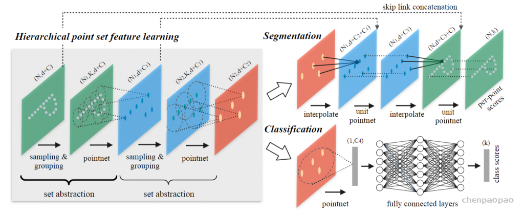
经过前半部分的encoder，我们得到的是global feature，或者是极少数点的表征（其实也就是global feature）

而如果做分割，我们需要的是point-wise feature，这可怎么办呢？

PointNet处理思路很简单，直接把global feature复制并与之前的local feature拼接，使得这个新point-wise feature能够获得一定程度的“邻域”信息。这种简单粗暴的方法显然并不能得到很discriminative的表征

别急，PointNet++来了。

PointNet++设计了一种反向插值的方法来实现上采样的decoder结构，通过反向插值和skip connection来获得discriminative point-wise feature：

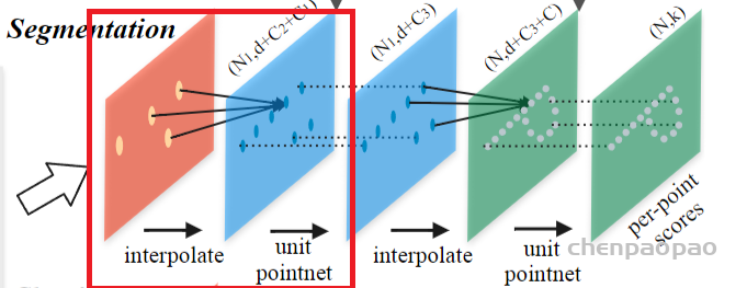
设红色矩形点集 P1 : N1∗C ，蓝色矩形点集 P2 : N2∗C2 ，因为decoder是上采样过程，因此 N2>N1

一、反向插值具体做法：

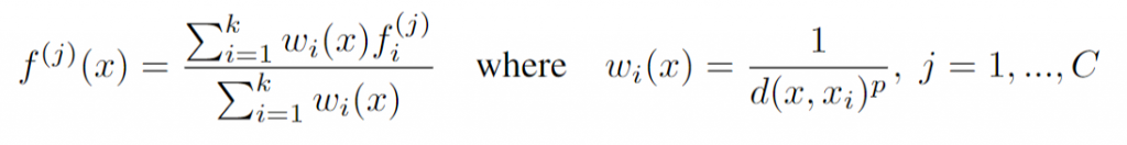
对于 P2 中的每个点 x ，找在原始点云坐标空间下， P1 中与其最接近的 k 个点 x1,…,xk

当前我们想通过反向插值的方式用较少的点把更多的点的特征插出来，实现上采样

此时 x1,…,xk 的特征我们是知道的，我们想得到 x 的特征。如上公式，实际上就是将 x1,…,xk 的特征加权求和，得到x的特征。其中这个权重是与x和 x1,…,xk 的距离成反向相关的，意思就是距离越远的点，对x特征的贡献程度越小。P2 中其他点以此类推，从而实现了特征的上采样回传

二、skip connection具体做法：

回传得到的point-wise feature是从decoder的上一层得到的，因此算是global级别的信息，这对于想得到discriminative还是不够，因为我们还缺少local级别的信息！！！

如上图就是我们反向插值只得到了 C2 ，但是我们还需要提供local级别信息的 C1 特征！！！

这时skip connection来了！！！

skip connection其实就是将之前encoder对应层的表征直接拼接了过来

因为上图中encoder蓝色矩形点集的 C1 表征是来自于规模更大的绿色矩形点集的表征，这在一定程度上其实是实现了local级别的信息

我们通过反向插值和skip connection在decoder中逐级上采样得到local + global point-wise feature，得到了discriminative feature，应用于分割任务。

2.3 loss

无论是分类还是分割应用，本质上都是分类问题，因此loss就是分类任务中常用的交叉熵loss

2.4 其他的问题

Q：PointNet++梯度是如何回传的？？？

A：PointNet++ fps实际上并没有参与梯度计算和反向传播。

可以理解成是PointNet++将点云进行不同规模的fps降采样，事先将这些数据准备好，再送到网络中去训练的

3 dataset and experiments

3.1 dataset

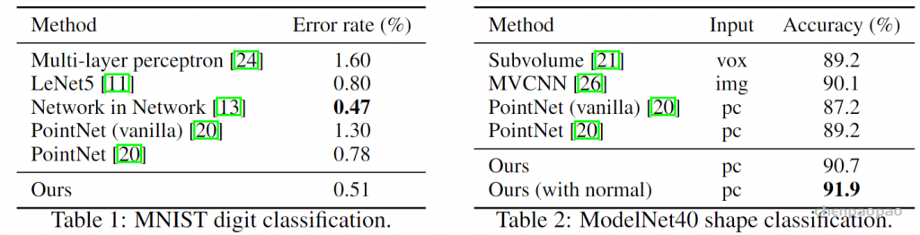
• MNIST: Images of handwritten digits with 60k training and 10k testing samples.（用于分类）
• ModelNet40: CAD models of 40 categories (mostly man-made). We use the official split with 9,843 shapes for training and 2,468 for testing. （用于分类）
• SHREC15: 1200 shapes from 50 categories. Each category contains 24 shapes which are mostly organic ones with various poses such as horses, cats, etc. We use five fold cross validation to acquire classification accuracy on this dataset. （用于分类）
• ScanNet: 1513 scanned and reconstructed indoor scenes. We follow the experiment setting in [5] and use 1201 scenes for training, 312 scenes for test. （用于分割）

3.2 experiments

主要关心的实验结果是2个：

1. ModelNet40分类结果
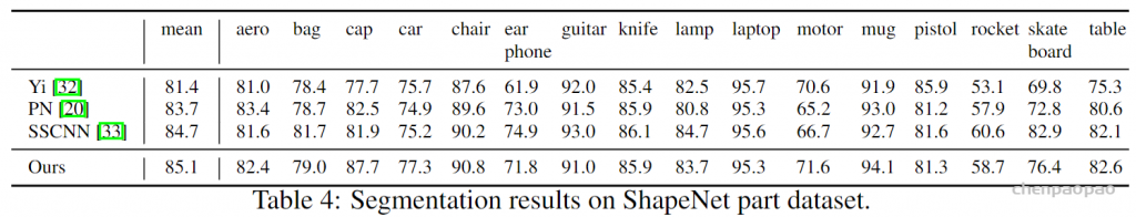
2. ShapeNet Part分割结果

4、 conclusion

PointNet++是PointNet的续作，在一定程度上弥补了PointNet的一些缺陷，表征网络基本和PN类似，还是MLP、 1∗1 卷积、pooling那一套，核心创新点在于设计了局部邻域的采样表征方法和这种多层次的encoder-decoder结合的网络结构。

第一次看到PointNet++网络结构，觉得设计得非常精妙，特别是设计了上采样和下采样的具体实现方法，并以此用于分割任务的表征，觉得设计得太漂亮了。但其实无论是分类还是分割任务，提升幅度较PointNet也就是1-2个点而已。

PointNet++，特别是其前半部分encoder，提供了非常好的表征网络，后面很多点云处理应用的论文都会使用到PointNet++作为它们的表征器。